Chapter 01 replaced a timetable’s signs with the table \(X_{ij}=s_i s_j\). There is a geometric way to read that table. A sign is a one-dimensional vector: \(1\) points one way along a line and \(-1\) points the other way. The product \(s_i s_j\) is their dot product.
What changes if each one-dimensional sign is replaced by a vector that may point anywhere in a plane or in a higher-dimensional space? Answering that question will show what kind of geometry a matrix can store. It does not alter the scheduling problem yet.
What can one table remember?
Place three unit vectors at a common origin:
Three vectors and the symbolic Gram matrix that records their geometry.
Put the vector coordinates in the rows of a matrix \(V\):
Multiplying \(V\) by its transpose creates a table containing every pairwise dot product:
\[
G=VV^T,
\qquad
G_{ij}=v_i^Tv_j.
\]
This table is called the Gram matrix of the vectors. Its entries have direct geometric meanings:
\[
\begin{aligned}
G_{ii}&=v_i^Tv_i=\lVert v_i\rVert_2^2,
&&\text{squared length of }v_i,\\
G_{ij}&=\lVert v_i\rVert_2\lVert v_j\rVert_2\cos\theta_{ij},
&&\text{angle between }v_i\text{ and }v_j,\\
\lVert v_i-v_j\rVert_2^2&=G_{ii}+G_{jj}-2G_{ij},
&&\text{squared distance between their endpoints.}
\end{aligned}
\]
For the pictured vectors, predict which off-diagonal entry is zero and which is negative. Then calculate the matrix.
The zero says \(v_2\) and \(v_3\) are perpendicular. The negative entry says the angle from \(v_1\) to \(v_3\) is obtuse. If the picture disappeared but \(G\) remained, its entries would retain all the lengths, angles, and pairwise distances shown above. This is the sense in which the matrix remembers the shape.
Can every symmetric table describe vectors?
Return to the impossible relationship table from Chapter 01:
It could not describe three signs because it claimed every pair occupied different slots. Could it at least be the Gram matrix of three vectors in a larger space?
If \(G=VV^T\), then for every vector of coefficients \(z\),
Therefore no real vectors can have \(Y\) as their Gram matrix. This motivates the defining test: a real symmetric matrix \(G\) is positive semidefinite (PSD) when
\[
z^TGz\ge0
\qquad\text{for every real vector }z.
\]
Every Gram matrix is PSD because a squared length cannot be negative. The converse is also true: every real symmetric PSD matrix is a Gram matrix. We will construct its vectors shortly.
For a symmetric matrix, the same condition can be checked through its eigenvalues:
\[
G\succeq0
\quad\Longleftrightarrow\quad
\text{every eigenvalue of }G\text{ is nonnegative}.
\]
PSD also does not mean entrywise nonnegative. The pictured Gram matrix contains the negative entry \(v_1^Tv_3=-0.8\) and is still PSD. Keep these properties separate: symmetry, the signs of individual entries, and positive semidefiniteness.
NoteGo further: Gram matrices
For a more formal linear-algebra treatment, the opening SDP sections of Vandenberghe and Boyd’s survey connect quadratic forms, eigenvalues, and matrix inequalities. This course continues with the computational and geometric route.
How far apart can two unit vectors point?
Suppose \(v_1\) and \(v_2\) are unit vectors. Their Gram matrix must have the form
Before calculating an eigenvalue, use the picture to answer two questions: what values can \(\cos\theta\) take, and what do the two vectors look like at the extreme values?
The dot product t moves from minus one to one as the angle between two unit vectors changes.
A dot product of \(1\) means the vectors coincide. A dot product of \(-1\) means they point in opposite directions. Both endpoint configurations lie on a single line. For \(-1<t<1\), the vectors span a plane.
The eigenvalues confirm the same interval:
\[
\lambda_1=1-t,
\qquad
\lambda_2=1+t.
\]
Both are nonnegative exactly when \(-1\le t\le1\). At \(t=-1\) or \(t=1\), one eigenvalue is zero and the matrix has rank one. In the interior, both eigenvalues are positive and the matrix has rank two.
M(t) = [1.0 t; t 1.0]for t in (-1.2, -1.0, 0.0, 0.5, 1.0, 1.2)println("t = $(lpad(t, 4)) λ = ",round.(eigvals(Symmetric(M(t))); digits =3))end
t = -1.2  λ = [-0.2, 2.2]
t = -1.0  λ = [0.0, 2.0]
t =  0.0  λ = [1.0, 1.0]
t =  0.5  λ = [0.5, 1.5]
t =  1.0  λ = [0.0, 2.0]
t =  1.2  λ = [-0.2, 2.2]
The values outside \([-1,1]\) produce a negative eigenvalue. No pair of real unit vectors can have those dot products.
Can the matrix redraw the vectors?
Start with the concrete matrix \(M(0.25)\). Choose the first unit vector as \(v_1=[1,0]^T\). Its dot product with the second vector must be \(0.25\), so the first coordinate of \(v_2\) must be \(0.25\). The unit-length requirement supplies the other coordinate:
Using \(v_1^T\) and \(v_2^T\) as the rows of \(V\) gives \(VV^T=M(0.25)\). We have redrawn one configuration directly from its Gram matrix.
For \(M(0.25)\), we found suitable coordinates by inspection. For a larger Gram matrix, an eigendecomposition constructs all those coordinates at once. If
then the rows of \(V\) have exactly the dot products stored in \(G\). This works because PSD makes every diagonal entry of \(\Lambda\) nonnegative, so every square root in \(\sqrt{\Lambda}\) is real.
If an eigenvalue \(\lambda_k\) is zero, column \(k\) of \(V=Q\sqrt{\Lambda}\) is an all-zero column. Removing that column changes none of the row dot products and therefore does not change \(VV^T\). This explains the earlier pictures: \(M(1)\) has one positive eigenvalue and can be drawn on a line, whereas \(M(0.25)\) has two positive eigenvalues and needs a plane.
G =M(0.25)factor =gram_factor(G; atol =1e-10)@assert factor * factor'≈ G atol =1e-10(factor =round.(factor; digits =3), reconstruction_error =norm(factor * factor'- G))
The helper performs the eigendecomposition, rejects eigenvalues below the chosen tolerance, and takes square roots of the accepted eigenvalues.
What part of the picture does the matrix forget?
The recovered coordinates are not unique. If \(R\) is an orthogonal matrix, so \(RR^T=I\), then
\[
(VR)(VR)^T
=VRR^TV^T
=VV^T.
\]
Multiplying by \(R\) rotates or reflects every vector together. Their coordinates change, but their lengths, angles, pairwise distances, and Gram matrix do not. Thus a Gram matrix remembers the geometry relative to the common origin while forgetting its orientation. Later, when coordinates have physical meaning, fixed anchors will supply a reference frame.
What if an eigenvalue is almost zero?
Floating-point calculations rarely produce exact zeros. Consider
This matrix has one positive eigenvalue near \(2\) and one negative eigenvalue near \(-2\times10^{-11}\). The negative eigenvalue proves that the matrix is not mathematically PSD; having eigenvalues of both signs makes it indefinite. A numerical routine may nevertheless accept the tiny negative value at a stated tolerance. “PSD within tolerance” is a computational judgment, not an exact mathematical claim.
We can now read PSD matrices as consistent records of vector geometry. Chapter 03 asks what the collection of all such matrices looks like and why that collection is suitable for optimization.
Try it yourself
Construct four unit vectors in \(\mathbb R^2\). Before multiplying, predict the diagonal and the largest possible rank of their Gram matrix.
Find a vector \(z\) proving that \(M(1.2)\) is not PSD without computing an eigenvalue.
Redraw two unit vectors whose Gram matrix is \(M(-0.6)\), then check their dot product in Julia.
Complete learner/02_matrices_as_geometry.jl and make every assertion pass.
Source Code
---title: "02. Can a matrix remember a shape?"engine: juliajulia: exeflags: ["--project=@."]---Chapter 01 replaced a timetable's signs with the table$X_{ij}=s_i s_j$. There is a geometric way to read that table. A sign is aone-dimensional vector: $1$ points one way along a line and $-1$ points theother way. The product $s_i s_j$ is their dot product.What changes if each one-dimensional sign is replaced by a vector that maypoint anywhere in a plane or in a higher-dimensional space? Answering thatquestion will show what kind of geometry a matrix can store. It does not alterthe scheduling problem yet.## What can one table remember?Place three unit vectors at a common origin: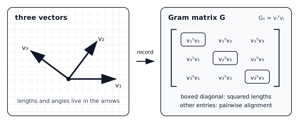{fig-alt="Three arrows share an origin. Vector v1 points right, v2 points up and right, and v3 points up and left. Beside them, a symbolic three by three Gram matrix labels entry i j as the dot product of vectors i and j; diagonal cells are marked as squared lengths."}Put the vector coordinates in the rows of a matrix $V$:$$V=\begin{bmatrix} 1 & 0\\ 0.6 & 0.8\\-0.8 & 0.6\end{bmatrix}.$$Multiplying $V$ by its transpose creates a table containing every pairwise dotproduct:$$G=VV^T,\qquadG_{ij}=v_i^Tv_j.$$This table is called the **Gram matrix** of the vectors. Its entries havedirect geometric meanings:$$\begin{aligned}G_{ii}&=v_i^Tv_i=\lVert v_i\rVert_2^2,&&\text{squared length of }v_i,\\G_{ij}&=\lVert v_i\rVert_2\lVert v_j\rVert_2\cos\theta_{ij},&&\text{angle between }v_i\text{ and }v_j,\\\lVert v_i-v_j\rVert_2^2&=G_{ii}+G_{jj}-2G_{ij},&&\text{squared distance between their endpoints.}\end{aligned}$$For the pictured vectors, predict which off-diagonal entry is zero and whichis negative. Then calculate the matrix.```{julia}#| label: first-gram-matrixusingLinearAlgebrausingLearnSDPV = [1.00.00.60.8-0.80.6]G = V * V'(G =round.(G; digits =3), squared_lengths =diag(G), eigenvalues =round.(eigvals(Symmetric(G)); digits =3))```The zero says $v_2$ and $v_3$ are perpendicular. The negative entry says theangle from $v_1$ to $v_3$ is obtuse. If the picture disappeared but $G$remained, its entries would retain all the lengths, angles, and pairwisedistances shown above. This is the sense in which the matrix remembers theshape.## Can every symmetric table describe vectors?Return to the impossible relationship table from Chapter 01:$$Y=\begin{bmatrix} 1 & -1 & -1\\-1 & 1 & -1\\-1 & -1 & 1\end{bmatrix}.$$It could not describe three signs because it claimed every pair occupieddifferent slots. Could it at least be the Gram matrix of three vectors in alarger space?If $G=VV^T$, then for every vector of coefficients $z$,$$z^TGz=z^TVV^Tz=\lVert V^Tz\rVert_2^2\ge 0.$$But with $z=[1,1,1]^T$,$$z^TYz=-3.$$Therefore no real vectors can have $Y$ as their Gram matrix. This motivatesthe defining test: a real symmetric matrix $G$ is **positive semidefinite(PSD)** when$$z^TGz\ge0\qquad\text{for every real vector }z.$$Every Gram matrix is PSD because a squared length cannot be negative. Theconverse is also true: every real symmetric PSD matrix is a Gram matrix. Wewill construct its vectors shortly.For a symmetric matrix, the same condition can be checked through itseigenvalues:$$G\succeq0\quad\Longleftrightarrow\quad\text{every eigenvalue of }G\text{ is nonnegative}.$$PSD also does not mean entrywise nonnegative. The pictured Gram matrix containsthe negative entry $v_1^Tv_3=-0.8$ and is still PSD. Keep these propertiesseparate: symmetry, the signs of individual entries, and positivesemidefiniteness.::: {.callout-note title="Go further: Gram matrices"}For a more formal linear-algebra treatment, the opening SDP sections of[Vandenberghe and Boyd's survey](https://web.stanford.edu/~boyd/papers/sdp.html)connect quadratic forms, eigenvalues, and matrix inequalities. This coursecontinues with the computational and geometric route.:::## How far apart can two unit vectors point?Suppose $v_1$ and $v_2$ are unit vectors. Their Gram matrix must have the form$$M(t)=\begin{bmatrix}1&t\\t&1\end{bmatrix},\qquadt=v_1^Tv_2=\cos\theta.$$Before calculating an eigenvalue, use the picture to answer two questions:what values can $\cos\theta$ take, and what do the two vectors look like atthe extreme values?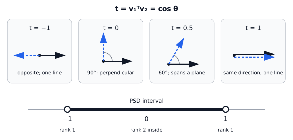{fig-alt="Four small vector diagrams show two unit vectors with dot products minus one, zero, one half, and one. At minus one the vectors point in opposite directions on one line; at zero they are perpendicular; at one half their angle is sixty degrees; at one they point in the same direction. A number line below marks the PSD interval from minus one to one, with rank one at the endpoints and rank two inside."}A dot product of $1$ means the vectors coincide. A dot product of $-1$ meansthey point in opposite directions. Both endpoint configurations lie on asingle line. For $-1<t<1$, the vectors span a plane.The eigenvalues confirm the same interval:$$\lambda_1=1-t,\qquad\lambda_2=1+t.$$Both are nonnegative exactly when $-1\le t\le1$. At $t=-1$ or $t=1$, oneeigenvalue is zero and the matrix has rank one. In the interior, botheigenvalues are positive and the matrix has rank two.```{julia}#| label: slice-eigenvaluesM(t) = [1.0 t; t 1.0]for t in (-1.2, -1.0, 0.0, 0.5, 1.0, 1.2)println("t = $(lpad(t, 4)) λ = ",round.(eigvals(Symmetric(M(t))); digits =3))end```The values outside $[-1,1]$ produce a negative eigenvalue. No pair of realunit vectors can have those dot products.## Can the matrix redraw the vectors?Start with the concrete matrix $M(0.25)$. Choose the first unit vector as$v_1=[1,0]^T$. Its dot product with the second vector must be $0.25$, so thefirst coordinate of $v_2$ must be $0.25$. The unit-length requirement suppliesthe other coordinate:$$v_2=\begin{bmatrix}0.25\\\sqrt{1-0.25^2}\end{bmatrix}.$$Using $v_1^T$ and $v_2^T$ as the rows of $V$ gives $VV^T=M(0.25)$. We haveredrawn one configuration directly from its Gram matrix.For $M(0.25)$, we found suitable coordinates by inspection. For a larger Grammatrix, an eigendecomposition constructs all those coordinates at once. If$$\begin{aligned}V&=Q\sqrt{\Lambda},\\VV^T&=Q\sqrt{\Lambda}\sqrt{\Lambda}Q^T =Q\Lambda Q^T =G.\end{aligned}$$then the rows of $V$ have exactly the dot products stored in $G$. This worksbecause PSD makes every diagonal entry of $\Lambda$ nonnegative, so everysquare root in $\sqrt{\Lambda}$ is real.If an eigenvalue $\lambda_k$ is zero, column $k$ of$V=Q\sqrt{\Lambda}$ is an all-zero column. Removing that column changes noneof the row dot products and therefore does not change $VV^T$. This explainsthe earlier pictures: $M(1)$ has one positive eigenvalue and can be drawn on aline, whereas $M(0.25)$ has two positive eigenvalues and needs a plane.```{julia}#| label: recover-factorG =M(0.25)factor =gram_factor(G; atol =1e-10)@assert factor * factor'≈ G atol =1e-10(factor =round.(factor; digits =3), reconstruction_error =norm(factor * factor'- G))```The helper performs the eigendecomposition, rejects eigenvalues below thechosen tolerance, and takes square roots of the accepted eigenvalues.## What part of the picture does the matrix forget?The recovered coordinates are not unique. If $R$ is an orthogonal matrix, so$RR^T=I$, then$$(VR)(VR)^T=VRR^TV^T=VV^T.$$Multiplying by $R$ rotates or reflects every vector together. Their coordinateschange, but their lengths, angles, pairwise distances, and Gram matrix do not.Thus a Gram matrix remembers the geometry relative to the common origin whileforgetting its orientation. Later, when coordinates have physical meaning,fixed anchors will supply a reference frame.## What if an eigenvalue is almost zero?Floating-point calculations rarely produce exact zeros. Consider```{julia}#| label: almost-psdalmost = [1.01.0+2e-11; 1.0+2e-111.0]λ =eigvals(Symmetric(almost))(eigenvalues = λ, accepted_at_1e_10 =minimum(λ) >=-1e-10, accepted_at_1e_12 =minimum(λ) >=-1e-12)```This matrix has one positive eigenvalue near $2$ and one negative eigenvaluenear $-2\times10^{-11}$. The negative eigenvalue proves that the matrix is notmathematically PSD; having eigenvalues of both signs makes it**indefinite**. A numerical routine may nevertheless accept the tiny negativevalue at a stated tolerance. “PSD within tolerance” is a computationaljudgment, not an exact mathematical claim.We can now read PSD matrices as consistent records of vector geometry. Chapter03 asks what the collection of all such matrices looks like and why thatcollection is suitable for optimization.## Try it yourself1. Construct four unit vectors in $\mathbb R^2$. Before multiplying, predict the diagonal and the largest possible rank of their Gram matrix.2. Find a vector $z$ proving that $M(1.2)$ is not PSD without computing an eigenvalue.3. Redraw two unit vectors whose Gram matrix is $M(-0.6)$, then check their dot product in Julia.4. Complete `learner/02_matrices_as_geometry.jl` and make every assertion pass.

