Correlation completion showed how PSD constraints control unknown inner products. Does that geometry transfer to a problem with a completely different surface story?
A collection of sensors may know distances to nearby sensors without knowing its own coordinates. This appears in wireless localization and more generally in graph realization. SDP-based methods have been developed for incomplete and noisy distance measurements. Biswas and Ye, 2004
This chapter uses a deliberately small, exact instance. Its purpose is to expose the Gram-matrix representation before dealing with missing or noisy ranges.
Five sensors connected by measured pairwise ranges.
The distance equation is linear in \(G\). Requiring \(G\succeq0\) guarantees that it describes some Euclidean vectors.
Distances alone cannot locate an absolute origin: adding the same translation to every sensor leaves every pairwise distance unchanged. We choose one representative by centering the positions,
\[
\sum_i p_i=0.
\]
If the position vectors are the rows of \(P\) and \(G=PP^T\), centering implies
\[
G\mathbf1=P(P^T\mathbf1)=0.
\]
We therefore require every row sum of \(G\) to be zero. This removes translation; rotation and reflection will remain.
In this first localization model every pairwise range is available. That makes the centered Gram matrix unique and lets us check the entire pipeline against known coordinates.
model =Model(Clarabel.Optimizer)set_silent(model)@variable(model, G[1:n, 1:n], PSD)@constraint(model, [i in1:n], sum(G[i, j] for j in1:n) ==0)@constraint( model, [i in1:n, j in (i +1):n], G[i, i] + G[j, j] -2G[i, j] == d²[i, j],)@objective(model, Min, 0)optimize!(model)Ĝ =Matrix(value.(G))(status =termination_status(model), minimum_eigenvalue =eigmin(Symmetric(Ĝ)), eigenvalues =round.(eigvals(Symmetric(Ĝ)); digits =7))
The recovered coordinates need not match the original coordinate columns. Rotation and reflection change coordinates but preserve the Gram geometry and all pairwise distances.
What exactly did feasibility establish?
The objective is zero, so this is a feasibility problem: every matrix satisfying the constraints is equally optimal. Complete exact distances plus centering make the Gram matrix unique in this instance. The coordinates are still not unique because rotation and reflection preserve that matrix.
With incomplete ranges, distinguish three questions:
Feasibility: does any Euclidean configuration match the measurements?
Uniqueness: do the constraints determine one Gram matrix?
Identifiability: after accounting for rigid motions, do they determine the physical configuration of interest?
A solver returning one feasible matrix answers only the first question unless additional structure proves the others.
What breaks with real measurements?
With only some ranges, many PSD completions may fit. With noisy ranges, exact equalities may be inconsistent. Practical formulations introduce residuals, weights, anchors, or objectives that choose among approximate realizations. The small feasibility problem above establishes the representation those models extend; it is not a deployment-ready localization system.
This detour has tested the Gram-matrix idea on physical geometry. We can now return to schedules and ask whether binary signs can be replaced by the same kind of vectors.
Try it yourself
Remove one distance constraint and determine whether the recovered missing distance is still unique.
Change one measured squared distance by 0.2. Inspect the termination status rather than attempting to read nonexistent variable values.
Generate points in three dimensions and predict the numerical rank of G.
Complete learner/05_geometry_from_distances.jl.
Source Code
---title: "05. Can distances reveal a map?"engine: juliajulia: exeflags: ["--project=@."]---Correlation completion showed how PSD constraints control unknown innerproducts. Does that geometry transfer to a problem with a completely differentsurface story?A collection of sensors may know distances to nearby sensors without knowingits own coordinates. This appears in wireless localization and more generallyin graph realization. SDP-based methods have been developed for incomplete andnoisy distance measurements. [Biswas and Ye, 2004](https://doi.org/10.1109/IPSN.2004.1307322)This chapter uses a deliberately small, exact instance. Its purpose is to exposethe Gram-matrix representation before dealing with missing or noisy ranges.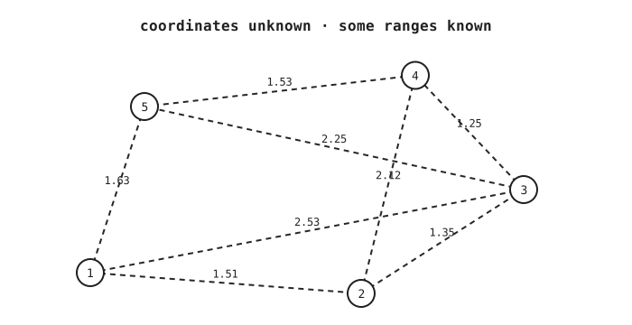{fig-alt="Five sensor nodes are connected by dashed lines labeled with measured distances."}::: {.callout-note title="Go further: localization"}The motivating method is developed in Biswas and Ye's primary paper,[Semidefinite Programming for Ad Hoc Wireless Sensor Network Localization](https://doi.org/10.1109/IPSN.2004.1307322).The paper includes anchors, incomplete measurements, and algorithmic issues thatour exact five-sensor experiment deliberately omits.:::## Can squared distances become linear?If the unknown position of sensor $i$ is $p_i$ and$G_{ij}=p_i^Tp_j$, then$$\lVert p_i-p_j\rVert_2^2=G_{ii}+G_{jj}-2G_{ij}.$$The distance equation is linear in $G$. Requiring $G\succeq0$ guarantees thatit describes some Euclidean vectors.Distances alone cannot locate an absolute origin: adding the same translationto every sensor leaves every pairwise distance unchanged. We choose onerepresentative by centering the positions,$$\sum_i p_i=0.$$If the position vectors are the rows of $P$ and $G=PP^T$, centering implies$$G\mathbf1=P(P^T\mathbf1)=0.$$We therefore require every row sum of $G$ to be zero. This removes translation;rotation and reflection will remain.```{julia}#| label: make-range-datausingJuMPusingClarabelusingLinearAlgebrapoints = [0.00.21.50.02.41.01.82.10.31.8]points .-=sum(points; dims =1) ./size(points, 1)n =size(points, 1)d² = [(sum(abs2, points[i, :] - points[j, :])) for i in1:n, j in1:n]```In this first localization model every pairwise range is available. That makesthe centered Gram matrix unique and lets us check the entire pipeline againstknown coordinates.```{julia}#| label: localization-sdpmodel =Model(Clarabel.Optimizer)set_silent(model)@variable(model, G[1:n, 1:n], PSD)@constraint(model, [i in1:n], sum(G[i, j] for j in1:n) ==0)@constraint( model, [i in1:n, j in (i +1):n], G[i, i] + G[j, j] -2G[i, j] == d²[i, j],)@objective(model, Min, 0)optimize!(model)Ĝ =Matrix(value.(G))(status =termination_status(model), minimum_eigenvalue =eigmin(Symmetric(Ĝ)), eigenvalues =round.(eigvals(Symmetric(Ĝ)); digits =7))```## Can we recover the hidden map?Only two eigenvalues should be meaningfully positive because the sensors livein the plane. Take the two leading eigenpairs to obtain coordinates.```{julia}#| label: recover-sensorsdecomposition =eigen(Symmetric(Ĝ))order =sortperm(decomposition.values; rev =true)keep = order[1:2]recovered = decomposition.vectors[:, keep] *Diagonal(sqrt.(max.(decomposition.values[keep], 0)))recovered_d² = [sum(abs2, recovered[i, :] - recovered[j, :]) for i in1:n, j in1:n](maximum_distance_error =maximum(abs.(recovered_d² - d²)), recovered_coordinates =round.(recovered; digits =4))```The recovered coordinates need not match the original coordinate columns.Rotation and reflection change coordinates but preserve the Gram geometry andall pairwise distances.## What exactly did feasibility establish?The objective is zero, so this is a feasibility problem: every matrix satisfyingthe constraints is equally optimal. Complete exact distances plus centeringmake the Gram matrix unique in this instance. The coordinates are still notunique because rotation and reflection preserve that matrix.With incomplete ranges, distinguish three questions:1. **Feasibility:** does any Euclidean configuration match the measurements?2. **Uniqueness:** do the constraints determine one Gram matrix?3. **Identifiability:** after accounting for rigid motions, do they determine the physical configuration of interest?A solver returning one feasible matrix answers only the first question unlessadditional structure proves the others.## What breaks with real measurements?With only some ranges, many PSD completions may fit. With noisy ranges, exactequalities may be inconsistent. Practical formulations introduce residuals,weights, anchors, or objectives that choose among approximate realizations. Thesmall feasibility problem above establishes the representation those modelsextend; it is not a deployment-ready localization system.This detour has tested the Gram-matrix idea on physical geometry. We can nowreturn to schedules and ask whether binary signs can be replaced by the samekind of vectors.## Try it yourself1. Remove one distance constraint and determine whether the recovered missing distance is still unique.2. Change one measured squared distance by `0.2`. Inspect the termination status rather than attempting to read nonexistent variable values.3. Generate points in three dimensions and predict the numerical rank of `G`.4. Complete `learner/05_geometry_from_distances.jl`.
