The audited SDP matrix is geometrically meaningful and numerically credible, but the registrar still cannot schedule a matrix. We need one sign—and therefore one time slot—for each course.
Factor the matrix into unit vectors \(v_i\). To recover signs, draw a random direction \(r\) and cut with the hyperplane through the origin:
A random hyperplane converts two SDP vectors into opposite signs.
Why should a random hyperplane work?
Let \(\theta_{ij}=\arccos(v_i^Tv_j)\) be the angle between two SDP vectors. Only the plane spanned by those vectors matters. A hyperplane through the origin is determined by its normal direction, and reversing that normal produces the same hyperplane, so the possible orientations occupy an angular range of length \(\pi\). Separating orientations occupy a range of length \(\theta_{ij}\). Their fraction is \(\theta_{ij}/\pi\).
Summing that separation probability over the weighted edges gives
The SDP assigns the same edge the contribution \(W_{ij}(1-\cos\theta_{ij})/2\). Goemans and Williamson bound the first expression against the second for every angle, giving the constant \(\alpha\approx0.87856\). For nonnegative edge weights, the expected rounded cut is at least \(\alpha\) times the true maximum-cut value.
The word expected matters. An individual random direction can do worse. Repeating the experiment and retaining the best feasible cut improves the observed result, while the SDP and dual bounds remain the certificates.
Changing the random direction can improve or worsen the feasible cut, but never invalidates it. Repetition is therefore a useful algorithmic choice rather than a proof technique.
The complete course pipeline: weighted graph, SDP vectors, and rounded cut.
For this ten-vertex teaching instance we can enumerate all distinct cuts and check how rounding performed. Enumeration is an evaluation tool here, not part of the scalable SDP method.
The rounded solution happens to reach the exact optimum on this graph. The SDP bound remains larger, which correctly reveals that the relaxation itself is not exact.
What schedule did geometry produce?
The vector of signs is useful only after translating it back to the original decision.
This final translation exposes the model’s scope. “Unresolved shared students” is an aggregate pairwise count, not necessarily the number of distinct people with a clash. The schedule still ignores rooms and other constraints listed in Chapter 00. A mathematically strong solution to the simplified model does not repair those omissions.
Can you own the complete pipeline?
Start from learner/10_relax_solve_round.jl and replace the exam-conflict graph by an unseen weighted graph with 12–18 vertices. Produce one reproducible report that:
explains what vertices and weights represent in your chosen setting;
constructs the Laplacian and SDP without calling maxcut_problem;
checks the matrix encoding on at least one known cut;
solves and audits the relaxation;
factors the Gram matrix and implements hyperplane rounding;
compares multiple trial budgets and a random-cut baseline;
reports a feasible cut, a valid upper bound, and their gap;
distinguishes observed numerical evidence from exact conclusions.
Possible settings include separating mutually interfering tasks, partitioning a small interaction network, or testing synthetic graph families. Choose one only when its edge weights have a defensible meaning; an unexplained random graph is acceptable for algorithm testing but should be described as synthetic.
At this point every link promised on the home page has now been built: the matrix is geometry, the geometry is a relaxation, duality explains the bound, audits qualify the computation, and rounding returns a feasible decision.
Source Code
---title: "10. Can geometry make a timetable?"engine: juliajulia: exeflags: ["--project=@."]---The audited SDP matrix is geometrically meaningful and numerically credible,but the registrar still cannot schedule a matrix. We need one sign—and thereforeone time slot—for each course.Factor the matrix into unit vectors $v_i$. To recover signs, draw a randomdirection $r$ and cut with the hyperplane through the origin:$$s_i=\begin{cases}+1,&v_i^Tr\ge0,\\-1,&v_i^Tr<0.\end{cases}$$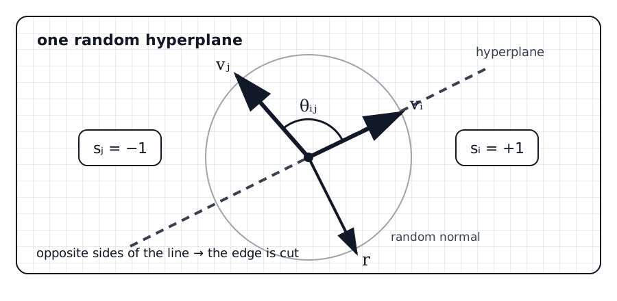{fig-alt="Two unit vectors extend from a common origin on opposite sides of a dashed line through the origin. A perpendicular arrow labeled r is the random normal direction. The vectors receive plus one and minus one signs, and the angle between them is labeled theta."}## Why should a random hyperplane work?Let $\theta_{ij}=\arccos(v_i^Tv_j)$ be the angle between two SDP vectors.Only the plane spanned by those vectors matters. A hyperplane through theorigin is determined by its normal direction, and reversing that normalproduces the same hyperplane, so the possible orientations occupy an angularrange of length $\pi$. Separating orientations occupy a range of length$\theta_{ij}$. Their fraction is $\theta_{ij}/\pi$.Summing that separation probability over the weighted edges gives$$\mathbb E[\operatorname{cut}]=\sum_{i<j}W_{ij}\frac{\theta_{ij}}{\pi}.$$The SDP assigns the same edge the contribution$W_{ij}(1-\cos\theta_{ij})/2$. Goemans and Williamson bound the first expressionagainst the second for every angle, giving the constant$\alpha\approx0.87856$. For nonnegative edge weights, the expected rounded cutis at least $\alpha$ times the true maximum-cut value.The word **expected** matters. An individual random direction can do worse.Repeating the experiment and retaining the best feasible cut improves theobserved result, while the SDP and dual bounds remain the certificates.::: {.callout-note title="Go further: the rounding guarantee"}Goemans and Williamson prove the approximation guarantee and extend the methodto related discrete problems in[Improved approximation algorithms for maximum cut and satisfiability problems](https://math.mit.edu/~goemans/PAPERS/maxcut-jacm.pdf).The proof is optional; the angle-by-angle comparison above is the part used inthis course.:::## Where are the vectors?```{julia}#| label: solve-final-sdpusingLearnSDPusingClarabelusingLinearAlgebrausingRandomusingStatisticsW =course_graph()problem =maxcut_problem(W)result =solve_sdp(problem, Clarabel.Optimizer)report =audit_solution(result.model, problem, result.numerical_X)V =gram_factor(Matrix(Symmetric(result.numerical_X)); atol =1e-7)@assert V * V'≈ result.numerical_X atol =1e-7(sdp_upper_bound =-report.primal_objective, factorization_error =norm(V * V'- result.numerical_X), effective_rank =count(>(1e-7), eigvals(Symmetric(result.numerical_X))))```## Can one line split them?```{julia}#| label: one-hyperplanerng =MersenneTwister(7)direction =randn(rng, size(V, 2))signs =ifelse.(V * direction .>=0, 1, -1)one_cut =cut_weight(W, signs)(signs, one_cut)```Changing the random direction can improve or worsen the feasible cut, but neverinvalidates it. Repetition is therefore a useful algorithmic choice rather thana proof technique.## What does repetition buy?```{julia}#| label: repeated-roundingrounded =round_maxcut( W, result.numerical_X; trials =500, rng =MersenneTwister(7),)(best_cut = rounded.weight, worst_trial =minimum(rounded.trial_weights), mean_trial =mean(rounded.trial_weights), sdp_upper_bound =-report.primal_objective, certified_relative_gap = (-report.primal_objective - rounded.weight) /-report.primal_objective)```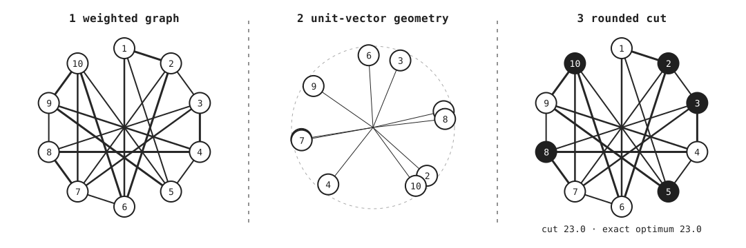{fig-alt="The exam-conflict graph becomes a configuration of vectors and then a cut with open and filled vertices on opposite sides."}For this ten-vertex teaching instance we can enumerate all distinct cuts andcheck how rounding performed. Enumeration is an evaluation tool here, not partof the scalable SDP method.```{julia}#| label: exact-small-checkexact =exact_maxcut(W)@assert rounded.weight <= exact.weight <=-report.primal_objective +1e-6(rounded = rounded.weight, exact = exact.weight, sdp_upper_bound =-report.primal_objective)```The rounded solution happens to reach the exact optimum on this graph. The SDPbound remains larger, which correctly reveals that the relaxation itself is notexact.## What schedule did geometry produce?The vector of signs is useful only after translating it back to the originaldecision.```{julia}#| label: interpret-rounded-schedulecourses = ["LA", "OPT", "STAT", "ML", "NUM","CTRL", "PROB", "GRAPH", "DATA", "SIGNAL"]slot_A = courses[rounded.signs .==1]slot_B = courses[rounded.signs .==-1]total_conflict_weight =sum(W) /2unresolved_weight = total_conflict_weight - rounded.weight(slot_A, slot_B, separated_shared_students =10* rounded.weight, unresolved_shared_students =10* unresolved_weight)```This final translation exposes the model's scope. “Unresolved shared students”is an aggregate pairwise count, not necessarily the number of distinct peoplewith a clash. The schedule still ignores rooms and other constraints listed inChapter 00. A mathematically strong solution to the simplified model does notrepair those omissions.## Can you own the complete pipeline?Start from `learner/10_relax_solve_round.jl` and replace the exam-conflict graph by anunseen weighted graph with 12–18 vertices. Produce one reproducible report that:1. explains what vertices and weights represent in your chosen setting;2. constructs the Laplacian and SDP without calling `maxcut_problem`;3. checks the matrix encoding on at least one known cut;4. solves and audits the relaxation;5. factors the Gram matrix and implements hyperplane rounding;6. compares multiple trial budgets and a random-cut baseline;7. reports a feasible cut, a valid upper bound, and their gap;8. distinguishes observed numerical evidence from exact conclusions.Possible settings include separating mutually interfering tasks, partitioning asmall interaction network, or testing synthetic graph families. Choose one onlywhen its edge weights have a defensible meaning; an unexplained random graph isacceptable for algorithm testing but should be described as synthetic.At this point every link promised on the home page has now been built: the matrix isgeometry, the geometry is a relaxation, duality explains the bound, auditsqualify the computation, and rounding returns a feasible decision.

