using XLSX, DataFrames, ReadStatTables
using Statistics, HypothesisTests
using CairoMakie
using DoingEconomics

CairoMakie.activate!(type = "svg")
use_doingecon_theme!()3. Measuring the effect of a sugar tax
Did Berkeley’s soda tax reach the shelf price?
In November 2014 Berkeley, California became the first US jurisdiction to tax distributors of sugar-sweetened beverages, at one cent per fluid ounce, effective January 2015. The tax falls on distributors, not shoppers — so whether it changes behaviour depends entirely on how much of it reaches the shelf.
- Part 3.1 — before-and-after comparisons of retail prices
- Part 3.2 — before-and-after comparisons against prices elsewhere
New concept: difference-in-differences, and the reason a before-and-after comparison on its own cannot carry the conclusion. Book pages: project, R walk-throughs, solutions.
The data
Two files, both from Silver et al. (2017), PLoS Medicine 14(4): e1002283.
| Store Price Survey | sps_public.xlsx — 2,175 shelf prices, 26 stores, 247 products, three waves |
| Point-of-sale prices | public_use_weighted_prices2.dta — 2,728 weighted monthly average prices, Berkeley vs elsewhere |
NoteTwo notes on this data vintage
The store survey’s third wave is labelled MAR2015 in the current file and MAR2016 in the book’s code, and supp is numeric here where the book compares it to the string "Standard". The published price means still reproduce exactly, so these are labelling changes rather than different observations.
The point-of-sale table is distributed as Stata .dta. CORE also offers it as .xls, but that is the legacy binary format XLSX.jl cannot read — it would need LibreOffice or Python to convert. The Stata original is what the book’s own walk-through 3.7 reads, and ReadStatTables.jl handles it directly, so no conversion step is needed.
dat = DataFrame(XLSX.readtable(rawpath("03", "sps_public.xlsx"), "Data"))

const STORE_TYPE = Dict(1 => "Large supermarket", 2 => "Small supermarket",
                        3 => "Pharmacy",          4 => "Gas station")
const WAVES = ["DEC2014", "JUN2015", "MAR2015"]

(rows = nrow(dat), columns = names(dat))
(rows = 2175, columns = ["store_id", "type", "store_type", "type2", "size", "price", "price_per_oz", "price_per_oz_c", "taxed", "supp", "time", "product_id"])The data dictionary ships as a second sheet:
DataFrame(XLSX.readtable(rawpath("03", "sps_public.xlsx"), "Data Dictionary"))12×3 DataFrame
| Row | Variable Name | Type | Description |
|---|---|---|---|
| String | String | String | |
| 1 | price | Num | Purchase Price |
| 2 | price_per_oz | Num | Price per ounce |
| 3 | price_per_oz_c | Num | Price per ounce cents |
| 4 | product_id | Num | Unique product identifier |
| 5 | size | Num | Total package size |
| 6 | store_id | Num | Unique store identifier |
| 7 | store_type | Num | Store Type: 1(Large Supermarket), 2(Small Supermarket), 3(Pharmacy), 4(Gas Station) |
| 8 | supp | Num | Supplemental(1) or standard(0) item in beverage panel |
| 9 | taxed | Num | Tax status |
| 10 | time | Text | Data collection month and year |
| 11 | type | Text | Product Type |
| 12 | type2 | Text | Specifies milk type or coconut water |
Part 3.1 — Before-and-after comparisons of retail prices
Q1. Stores and products
The paper’s S1 Text describes the survey: fieldworkers visited a fixed panel of Berkeley stores and recorded the shelf price and package size of a defined list of beverages, in three waves. Prices are converted to cents per fluid ounce so that packages of different sizes are comparable — the tax is levied per ounce, so per-ounce price is the quantity the policy acts on.
(stores = length(unique(dat.store_id)),
 products = length(unique(dat.product_id)),
 waves = sort(unique(dat.time)))
(stores = 26, products = 247, waves = ["DEC2014", "JUN2015", "MAR2015"])26 stores — matching the paper’s S1 Text — and 247 products.
Q2. Three frequency tables
"""Count rows by `rowvar` across the two compared waves, with a total column."""
function wave_table(df, rowvar; waves = ["DEC2014", "JUN2015"])
    keys = sort(unique(df[!, rowvar]), by = string)
    out = DataFrame(rowvar => keys)
    for w in waves
        out[!, w] = [sum((df[!, rowvar] .== k) .& (df.time .== w)) for k in keys]
    end
    return out
end

store_counts = wave_table(dat, :store_type)
store_counts.label = [STORE_TYPE[t] for t in store_counts.store_type]
select(store_counts, :store_type, :label, :DEC2014, :JUN2015)
4×4 DataFrame
| Row | store_type | label | DEC2014 | JUN2015 |
|---|---|---|---|---|
| Int64 | String | Int64 | Int64 | |
| 1 | 1 | Large supermarket | 177 | 209 |
| 2 | 2 | Small supermarket | 407 | 391 |
| 3 | 3 | Pharmacy | 87 | 102 |
| 4 | 4 | Gas station | 73 | 96 |
Observation counts are close but not equal between waves — 744 in December against 798 in June. Products go in and out of stock, so a store visited twice does not yield the same basket twice. That is the fact Q3’s filter exists to handle.
taxed_counts = DataFrame(store_type = 1:4,
                         label = [STORE_TYPE[t] for t in 1:4])
for (col, tx) in (("non_taxed", 0), ("taxed", 1))
    taxed_counts[!, col] = [sum((dat.store_type .== t) .& (dat.taxed .== tx)) for t in 1:4]
end
taxed_counts.share_taxed = round.(
    100 .* taxed_counts.taxed ./ (taxed_counts.taxed .+ taxed_counts.non_taxed), digits = 1)

taxed_counts
4×5 DataFrame
| Row | store_type | label | non_taxed | taxed | share_taxed |
|---|---|---|---|---|---|
| Int64 | String | Int64 | Int64 | Float64 | |
| 1 | 1 | Large supermarket | 291 | 253 | 46.5 |
| 2 | 2 | Small supermarket | 542 | 583 | 51.8 |
| 3 | 3 | Pharmacy | 132 | 130 | 49.6 |
| 4 | 4 | Gas station | 109 | 135 | 55.3 |
Roughly 60% of observations are taxed beverages in every store type, so the taxed/non-taxed split is not confounded with store type.
wave_table(dat, :type)13×3 DataFrame
| Row | type | DEC2014 | JUN2015 |
|---|---|---|---|
| String | Int64 | Int64 | |
| 1 | ENERGY | 56 | 58 |
| 2 | ENERGY-DIET | 49 | 54 |
| 3 | JUICE | 70 | 64 |
| 4 | JUICE DRINK | 19 | 17 |
| 5 | MILK | 63 | 61 |
| 6 | SODA | 239 | 262 |
| 7 | SODA-DIET | 128 | 174 |
| 8 | SPORT | 11 | 16 |
| 9 | SPORT-DIET | 2 | 2 |
| 10 | TEA | 52 | 45 |
| 11 | TEA-DIET | 6 | 6 |
| 12 | WATER | 48 | 38 |
| 13 | WATER-SWEET | 1 | 1 |
Soda dominates (239 in December, 262 in June) and diet soda is second; sport drinks and sweetened water have a handful of observations each. The survey was designed around the beverages the tax targets, and stocks more of what stores actually carry — so the counts reflect both the sampling design and shelf reality.
Q3. Conditional means
The paper’s method, which the question asks us to follow: keep only products present in all three waves at the same store, and only non-supplementary items (supp == 0).
The reason is Q2’s finding. Comparing the December mean against the June mean over different baskets measures two things at once — the price change, and the change in which products were on the shelf. Restricting to a matched basket removes the second.
The book does this with a nested loop over every store × product pair. groupby states the same condition directly and does it in one pass:
# Keep (store, product) pairs observed in all three waves.
complete = combine(groupby(dat, [:store_id, :product_id]),
                   :time => (t -> length(unique(t)) == 3) => :all_waves)

balanced = innerjoin(dat, complete[complete.all_waves, [:store_id, :product_id]];
                     on = [:store_id, :product_id])
balanced = balanced[balanced.supp .== 0, :]

(rows = nrow(balanced),
 stores = length(unique(balanced.store_id)),
 products = length(unique(balanced.product_id)))
(rows = 939, stores = 24, products = 55)939 observations, 24 stores, 55 products — a much smaller but genuinely comparable sample.
price_means = combine(
    groupby(balanced, [:taxed, :store_type, :time]),
    nrow => :n,
    :price_per_oz_c => (x -> round(mean(x), digits = 2)) => :mean_cents_per_oz)

sort!(price_means, [:taxed, :store_type, :time])
price_means.store = [STORE_TYPE[t] for t in price_means.store_type]
select(price_means, :taxed, :store, :time, :n, :mean_cents_per_oz)
24×5 DataFrame
| Row | taxed | store | time | n | mean_cents_per_oz |
|---|---|---|---|---|---|
| Int64 | String | String | Int64 | Float64 | |
| 1 | 0 | Large supermarket | DEC2014 | 36 | 11.19 |
| 2 | 0 | Large supermarket | JUN2015 | 36 | 11.48 |
| 3 | 0 | Large supermarket | MAR2015 | 36 | 11.7 |
| 4 | 0 | Small supermarket | DEC2014 | 70 | 13.67 |
| 5 | 0 | Small supermarket | JUN2015 | 70 | 13.82 |
| 6 | 0 | Small supermarket | MAR2015 | 70 | 13.37 |
| 7 | 0 | Pharmacy | DEC2014 | 18 | 15.2 |
| 8 | 0 | Pharmacy | JUN2015 | 18 | 16.08 |
| 9 | 0 | Pharmacy | MAR2015 | 18 | 15.44 |
| 10 | 0 | Gas station | DEC2014 | 12 | 16.94 |
| 11 | 0 | Gas station | JUN2015 | 12 | 16.96 |
| 12 | 0 | Gas station | MAR2015 | 12 | 17.04 |
| 13 | 1 | Large supermarket | DEC2014 | 36 | 15.62 |
| 14 | 1 | Large supermarket | JUN2015 | 36 | 16.93 |
| 15 | 1 | Large supermarket | MAR2015 | 36 | 16.68 |
| 16 | 1 | Small supermarket | DEC2014 | 101 | 15.85 |
| 17 | 1 | Small supermarket | JUN2015 | 101 | 16.0 |
| 18 | 1 | Small supermarket | MAR2015 | 101 | 15.49 |
| 19 | 1 | Pharmacy | DEC2014 | 18 | 18.18 |
| 20 | 1 | Pharmacy | JUN2015 | 18 | 19.08 |
| 21 | 1 | Pharmacy | MAR2015 | 18 | 18.63 |
| 22 | 1 | Gas station | DEC2014 | 22 | 19.41 |
| 23 | 1 | Gas station | JUN2015 | 22 | 20.34 |
| 24 | 1 | Gas station | MAR2015 | 22 | 19.24 |
Every value reproduces the book’s published solutions exactly. Note n is identical across waves within each cell (36, 36, 36 for large supermarkets) — that is the balanced panel working.
Two patterns, before calculating anything:
- Taxed beverages cost more per ounce than untaxed ones in every store type and every wave, including December 2014, before the tax applied. Sodas are sold in smaller, pricier-per-ounce formats than milk or juice.
- Prices rise between December and June for taxed beverages, and rise much less for untaxed ones.
Could we assess the tax by comparing taxed against untaxed prices in a single period? No. The first pattern is the reason: taxed and untaxed beverages already differed by 4–5 cents per ounce before the tax existed. That gap measures what kind of drinks they are, not the tax. Only the change in the gap is informative.
Q4. Price changes
changes = unstack(select(price_means, :taxed, :store_type, :time, :mean_cents_per_oz),
                  [:taxed, :store_type], :time, :mean_cents_per_oz)
changes.change = round.(changes.JUN2015 .- changes.DEC2014, digits = 2)
changes.store = [STORE_TYPE[t] for t in changes.store_type]

select(sort(changes, [:taxed, :store_type]),
       :taxed, :store, :DEC2014, :JUN2015, :change)
8×5 DataFrame
| Row | taxed | store | DEC2014 | JUN2015 | change |
|---|---|---|---|---|---|
| Int64 | String | Float64? | Float64? | Float64 | |
| 1 | 0 | Large supermarket | 11.19 | 11.48 | 0.29 |
| 2 | 0 | Small supermarket | 13.67 | 13.82 | 0.15 |
| 3 | 0 | Pharmacy | 15.2 | 16.08 | 0.88 |
| 4 | 0 | Gas station | 16.94 | 16.96 | 0.02 |
| 5 | 1 | Large supermarket | 15.62 | 16.93 | 1.31 |
| 6 | 1 | Small supermarket | 15.85 | 16.0 | 0.15 |
| 7 | 1 | Pharmacy | 18.18 | 19.08 | 0.9 |
| 8 | 1 | Gas station | 19.41 | 20.34 | 0.93 |
fig = Figure(size = (760, 440))
ax = Axis(fig[1, 1];
          title = "Taxed beverages rose more than untaxed ones",
          ylabel = "Change in price (cents per ounce)",
          xticks = (1:4, ["Large\nsupermarket", "Small\nsupermarket",
                          "Pharmacy", "Gas\nstation"]))
hlines!(ax, 0; color = BASELINE, linewidth = 1)

for (i, tx) in enumerate((0, 1))
    rows = sort(changes[changes.taxed .== tx, :], :store_type)
    xs = collect((1:4) .+ (i - 1.5) * 0.2)
    barplot!(ax, xs, rows.change; width = 0.16, color = series_color(i),
             label = tx == 1 ? "Taxed" : "Untaxed")
    for (x, v) in zip(xs, rows.change)
        text!(ax, x, v; text = string(v), fontsize = 10,
              align = (:center, v < 0 ? :top : :bottom), offset = (0, v < 0 ? -4 : 4))
    end
end

Legend(fig[1, 2], ax; framevisible = false)
fig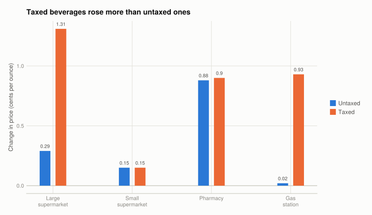
The large-supermarket contrast is the clearest: taxed beverages up 1.31 cents per ounce against 0.29 for untaxed. Gas stations show the opposite sign, on 22 taxed observations.
Q5. Are the changes statistically distinguishable?
Because the panel is balanced, each store-product appears in both waves, so the price change can be computed per item and tested as a paired difference.
wide = unstack(select(balanced, :store_id, :product_id, :store_type, :taxed,
                      :time, :price_per_oz_c),
               [:store_id, :product_id, :store_type, :taxed], :time, :price_per_oz_c)
wide.diff = wide.JUN2015 .- wide.DEC2014

tests = DataFrame(store_type = Int[], taxed = Int[], n = Int[],
                  mean_change = Float64[], p_value = Float64[])
for st in 1:4, tx in (0, 1)
    # `unstack` widens the element type to admit missing even when the balanced
    # panel leaves none, and the test needs a concrete Float64 vector.
    d = collect(skipmissing(wide[(wide.store_type .== st) .& (wide.taxed .== tx), :diff]))
    t = OneSampleTTest(d)
    push!(tests, (st, tx, length(d), round(mean(d), digits = 3),
                  round(pvalue(t), digits = 4)))
end
tests.store = [STORE_TYPE[t] for t in tests.store_type]
select(tests, :store, :taxed, :n, :mean_change, :p_value)
8×5 DataFrame
| Row | store | taxed | n | mean_change | p_value |
|---|---|---|---|---|---|
| String | Int64 | Int64 | Float64 | Float64 | |
| 1 | Large supermarket | 0 | 36 | 0.288 | 0.0777 |
| 2 | Large supermarket | 1 | 36 | 1.312 | 0.0 |
| 3 | Small supermarket | 0 | 70 | 0.146 | 0.3678 |
| 4 | Small supermarket | 1 | 101 | 0.144 | 0.429 |
| 5 | Pharmacy | 0 | 18 | 0.88 | 0.3645 |
| 6 | Pharmacy | 1 | 18 | 0.897 | 0.3556 |
| 7 | Gas station | 0 | 12 | 0.029 | 0.9399 |
| 8 | Gas station | 1 | 22 | 0.925 | 0.3305 |
Taxed beverages in large supermarkets and pharmacies show increases that are unlikely under no real change. Untaxed beverages mostly do not. The cell sizes are small — 18 to 36 items — so these are indicative rather than decisive.
But no p-value here can establish that the tax caused the rise. Every comparison in Part 3.1 is Berkeley in December against Berkeley in June. Anything else that moved prices over those six months — supplier costs, inflation, seasonal demand — is inside the estimate. That is what Part 3.2 addresses.
Part 3.2 — Comparison with prices elsewhere
pos = DataFrame(readstat(rawpath("03", "public_use_weighted_prices2.dta")))
pos = dropmissing(pos, :price)

# Stata string columns arrive as String15/String31; plain String compares cleanly.
for c in (:location, :beverage_group, :tax)
    pos[!, c] = String.(pos[!, c])
end
pos.date = pos.year .+ (pos.month .- 1) ./ 12

(rows = nrow(pos), years = extrema(pos.year),
 groups = sort(unique(pos.beverage_group)))
(rows = 2696, years = (2013.0, 2016.0), groups = ["fruit drinks/flavored waters", "milk", "milk substitutes", "soda", "water"])Q1. Were the comparison stores well chosen?
The comparison stores are in adjacent non-Berkeley areas. What makes a comparison group suitable is not that it resembles Berkeley on every measure, but that its prices would have moved the same way had Berkeley not taxed. The pre-tax period is what evidences that, and Figure 2 below is the test: two years of prices before the tax, and the question of whether the two locations track each other.
The paper’s S5 Table shows the comparison stores differ from Berkeley’s on neighbourhood characteristics — income and demographics. That matters for levels, which need not match, and matters much less for trends, which do.
Q2. Prices by location and tax status
monthly = combine(groupby(pos, [:year, :month, :date, :location, :tax]),
                  :price => mean => :price)
sort!(monthly, :date)

# `unstack` spreads a single column, so the two-way tax x location split becomes
# one series label first.
labelled = transform(monthly,
    [:tax, :location] => ByRow((t, l) -> "$t, $l") => :series)

first(unstack(select(labelled, :year, :month, :series, :price),
              [:year, :month], :series, :price), 8)
8×6 DataFrame
| Row | year | month | Non-taxed, Berkeley | Non-taxed, Non-Berkeley | Taxed, Berkeley | Taxed, Non-Berkeley |
|---|---|---|---|---|---|---|
| Float64 | Float64 | Float64? | Float64? | Float64? | Float64? | |
| 1 | 2013.0 | 1.0 | 5.72248 | 5.34864 | 8.6928 | 7.99157 |
| 2 | 2013.0 | 2.0 | 5.80647 | 5.36386 | 8.65457 | 8.18088 |
| 3 | 2013.0 | 3.0 | 5.85825 | 5.42451 | 8.82269 | 8.18687 |
| 4 | 2013.0 | 4.0 | 5.85834 | 5.64346 | 9.02207 | 8.24645 |
| 5 | 2013.0 | 5.0 | 5.79133 | 5.18173 | 8.67854 | 7.75679 |
| 6 | 2013.0 | 6.0 | 5.76184 | 5.03197 | 8.57345 | 7.4264 |
| 7 | 2013.0 | 7.0 | 5.90282 | 5.09817 | 8.23329 | 7.19362 |
| 8 | 2013.0 | 8.0 | 5.83173 | 5.08038 | 8.82165 | 7.48876 |
fig = Figure(size = (900, 440))
Label(fig[0, 1:2], "Berkeley's taxed prices step up after January 2015; untaxed prices don't";
      fontsize = 15, font = :bold, color = INK, halign = :left,
      tellwidth = false, padding = (0, 0, 8, 0))

ylims = extrema(monthly.price) .+ (-0.4, 0.4)

panels = ["Taxed", "Non-taxed"]

# Build the axes up front rather than capturing one from inside the loop: at top
# level, assigning to an outer name inside `for` creates a local under Julia's
# soft scope, so the captured reference would still be `nothing` in a script.
axs = [Axis(fig[1, i]; title = "$(panels[i]) beverages", xlabel = "Year",
            ylabel = i == 1 ? "Mean price (cents per ounce)" : "",
            limits = (nothing, ylims)) for i in eachindex(panels)]

for (i, ax) in enumerate(axs)
    vlines!(ax, 2015.0; color = BASELINE, linewidth = 1)
    for (j, loc) in enumerate(("Berkeley", "Non-Berkeley"))
        s = monthly[(monthly.tax .== panels[i]) .& (monthly.location .== loc), :]
        lines!(ax, s.date, s.price; color = series_color(j), label = loc)
    end
    i == 2 && hideydecorations!(ax; grid = false)
end

# One shared legend from the left panel, rather than the same two entries twice.
Legend(fig[2, 1:2], first(axs); orientation = :horizontal, framevisible = false)
colgap!(fig.layout, 28)
fig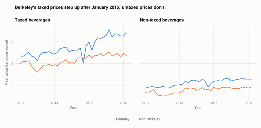
Untaxed beverages: the two locations move broadly together, with Berkeley about 0.6 cents higher throughout. Berkeley does drift up slightly faster over the period — Q3 puts a number on it — but the panels stay close and there is no step at January 2015.
Taxed beverages: the two move together through 2013 and 2014, then separate once the tax takes effect. Berkeley steps up sharply; the comparison areas continue on roughly their previous path. The gap goes from about 1.0 cents to about 1.7.
That pre-tax co-movement is what licenses the comparison: two series that tracked each other for two years and diverge when the policy changes is a far stronger basis than Berkeley rising alone.
Is it reasonable to conclude the tax affected prices? Yes — the timing and the size of the step in the taxed panel, with no matching step in the untaxed one, are hard to explain otherwise. But the untaxed panel is a qualified control rather than a perfect one: Berkeley’s untaxed prices also rose a little faster than its neighbours’, so some general Berkeley drift is present. Q3 quantifies how much that matters.
Q3. Difference-in-differences
The chart’s logic as a number. Take the change in Berkeley, subtract the change outside Berkeley, and what remains is the part not explained by whatever moved prices in both places:
"""Mean price in a cell, using the book's windows: pre through Dec 2014, post from Mar 2015."""
function cell_mean(df, loc, tx, period)
    s = df[(df.location .== loc) .& (df.tax .== tx), :]
    rows = period === :pre ? s[s.date .< 2015.0, :] : s[s.date .>= 2015.0 + 2 / 12, :]
    return mean(rows.price)
end

did = DataFrame(tax = String[], berkeley_pre = Float64[], berkeley_post = Float64[],
                other_pre = Float64[], other_post = Float64[])
for tx in ("Taxed", "Non-taxed")
    push!(did, (tx,
        cell_mean(pos, "Berkeley", tx, :pre),  cell_mean(pos, "Berkeley", tx, :post),
        cell_mean(pos, "Non-Berkeley", tx, :pre), cell_mean(pos, "Non-Berkeley", tx, :post)))
end

did.berkeley_change = did.berkeley_post .- did.berkeley_pre
did.other_change = did.other_post .- did.other_pre
did.diff_in_diff = did.berkeley_change .- did.other_change

select(transform(did, names(did, Float64) .=> ByRow(x -> round(x, digits = 3)); renamecols = false),
       :tax, :berkeley_change, :other_change, :diff_in_diff)
2×4 DataFrame
| Row | tax | berkeley_change | other_change | diff_in_diff |
|---|---|---|---|---|
| String | Float64 | Float64 | Float64 | |
| 1 | Taxed | 1.549 | 0.814 | 0.735 |
| 2 | Non-taxed | 0.474 | 0.342 | 0.132 |
For taxed beverages the difference-in-differences is +0.74 cents per ounce against a tax of exactly 1 cent — roughly 74% pass-through to the shelf. Distributors and retailers absorbed about a quarter of it. That is in line with the published estimates for Berkeley, and it is the substantive answer to the project’s question: the tax reached the shelf, but not all of it did.
For untaxed beverages the same calculation gives +0.13. Small next to 0.74, but not zero — and the test below says it is not noise either. That matters for how much weight the 0.74 can carry, so it is worth being precise rather than treating the untaxed row as a clean null.
# Berkeley's post-tax deviation from the comparison areas, month by month. Testing
# whether the gap widened rather than comparing raw prices removes the level
# difference between the two locations.
function monthly_gap(tx)
    b = monthly[(monthly.tax .== tx) .& (monthly.location .== "Berkeley"), :]
    o = monthly[(monthly.tax .== tx) .& (monthly.location .== "Non-Berkeley"), :]
    j = innerjoin(select(b, :date, :price => :berkeley),
                  select(o, :date, :price => :other); on = :date)
    j.gap = j.berkeley .- j.other
    return j
end

gap_tests = DataFrame(tax = String[], gap_pre = Float64[], gap_post = Float64[],
                      widening = Float64[], p_value = Float64[])
for tx in ("Taxed", "Non-taxed")
    j = monthly_gap(tx)
    pre = j[j.date .< 2015.0, :gap]
    post = j[j.date .>= 2015.0 + 2 / 12, :gap]
    push!(gap_tests, (tx, round(mean(pre), digits = 3), round(mean(post), digits = 3),
                      round(mean(post) - mean(pre), digits = 3),
                      round(pvalue(UnequalVarianceTTest(post, pre)), digits = 5)))
end

gap_tests
2×5 DataFrame
| Row | tax | gap_pre | gap_post | widening | p_value |
|---|---|---|---|---|---|
| String | Float64 | Float64 | Float64 | Float64 | |
| 1 | Taxed | 0.973 | 1.725 | 0.752 | 0.0 |
| 2 | Non-taxed | 0.637 | 0.773 | 0.136 | 0.00303 |
The taxed gap widens by 0.75 cents per ounce with a p-value of essentially zero. The untaxed gap widens by 0.14 with p = 0.003 — small, but statistically distinguishable from no change.
That untaxed result is a problem for the clean story, and worth taking seriously. The difference-in-differences rests on the comparison areas standing in for what Berkeley would have done anyway. Untaxed drinks, which the tax never touched, should therefore show no widening. They show a little. So something besides the tax was pushing Berkeley’s beverage prices up relative to its neighbours over this period.
Two readings, and the data here cannot separate them:
- A Berkeley-wide price drift. If whatever moved untaxed prices moved taxed ones equally, the tax effect is nearer 0.74 − 0.13 ≈ 0.6 cents per ounce, or 60% pass-through.
- A composition or measurement difference specific to untaxed drinks, in which case 0.74 stands.
Either way the qualitative conclusion survives: 0.13 is small beside 0.75, and the taxed widening is roughly five times larger and begins when the tax does. But the honest interval on pass-through is something like 60–75%, not a point estimate.
What the p-values do and do not tell us. They address one question: could a difference this size arise from ordinary month-to-month variation. They say nothing about whether the comparison group was well chosen — and the untaxed row is precisely where that assumption shows a crack. A badly chosen comparison area would still produce a confident p-value, for a meaningless estimate. The p-value tests the difference, not the design.
Q4. Consumption behaviour
The paper reports sugar-sweetened beverage sales falling roughly 10% in Berkeley while rising slightly in the comparison areas, with no fall in total beverage calories sold and a rise in water sales — consistent with substitution toward untaxed drinks rather than drinking less overall.
Three explanations consistent with a ~1 cent per ounce price rise producing that:
- Substitution, not abstention. The tax changes relative prices within the category. Water and milk became cheaper relative to soda, and that is the margin shoppers moved on.
- Cross-border shopping. Berkeley is small and bordered by untaxed cities. Some of the sales decline is purchases relocating rather than consumption falling — which is why the sales figures are weaker evidence about consumption than they first appear.
- Salience beyond price. The tax was a publicised local campaign. Some response may be to the message rather than to the cent.
Q5. Strengths and limitations
Strengths. A genuine policy change rather than a laboratory manipulation; a comparison group whose pre-tax prices track Berkeley’s for two years; two independent data sources — hand-collected shelf prices and point-of-sale records — pointing the same way.
Limitations, most consequential first, with what would address each:
- The untaxed control is not perfectly parallel. Berkeley’s untaxed prices rose 0.13 cents per ounce faster than the comparison areas’ (Q3), which is small but detectable. Pass-through is therefore bounded at roughly 60–75% rather than pinned at one number. More pre-tax years, or several comparison areas rather than one aggregate, would tighten it.
- 26 stores, and a matched basket of 55 products. Q3’s balanced panel bought comparability at the cost of sample size, and cells of 18 observations support weak inference. A larger store panel is the only fix.
- Berkeley is one small city. It is unusually affluent, politically distinctive, and surrounded by untaxed neighbours. None of that transfers automatically to a larger or poorer jurisdiction. Later taxes in Philadelphia, Seattle and Mexico are the replication.
- Cross-border shopping contaminates the comparison in both directions. If Berkeley shoppers buy soda outside the city, sales fall in Berkeley and rise in the comparison area, which inflates the estimated difference.
- Shelf prices are not transaction prices. Promotions, multi-buys and loyalty discounts are invisible in a shelf survey. Scanner data covers this and is what the second file provides.
- Six months is short. Pass-through can keep adjusting as contracts are renegotiated, so an estimate at six months need not be the long-run one.
Q6. Designing the experiment
With authority over two neighbouring towns, the design problem is to get comparability by construction rather than by argument.
- Randomise which town is taxed. With only two towns randomisation cannot balance characteristics, so it does not solve much on its own — but it does remove the worst threat, which is a town being selected for taxation because of its consumption patterns.
- Measure both towns for at least a year beforehand. This is the most valuable single step. Pre-treatment data is what lets you verify parallel trends instead of assuming them, and it is exactly what makes Figure 2 persuasive.
- Choose non-adjacent towns, or measure the border. Adjacency is what makes cross-border shopping possible. If the towns must be neighbours, survey stores by distance from the border so leakage can be estimated rather than ignored.
- Track untaxed products in the same stores. They are the within-experiment control: a spurious local shock moves them too, and a real tax does not.
- Announce and implement on a known date, and record prices monthly on both sides of it, so the timing of any change can be attributed rather than inferred.
- Collect transaction data, not just shelf prices, and total beverage volume rather than only taxed volume — otherwise substitution toward untaxed drinks reads as a fall in consumption.
The structural point is the one Part 3.1 illustrated by falling short of it: a before-and-after comparison measures the policy plus everything else that changed. A comparison group that would have moved the same way is what separates them, and pre-treatment data is the only way to know whether you have one.
What this project covered
| Concept | Where | In Julia |
|---|---|---|
| Reading a named Excel sheet | Setup | XLSX.readtable(path, "Data") |
| Reading a Stata file | Part 3.2 | readstat(path) (ReadStatTables.jl) |
| Frequency tables across waves | Q3.2 | groupby + counts, unstack |
| Balanced panel construction | Q3.3 | groupby + length(unique(t)) == 3, innerjoin |
| Conditional means | Q3.3 | combine(groupby(df, [...]), col => mean) |
| Long to wide | Q3.4 | unstack(df, keys, :time, :value) |
| Paired t-test on differences | Q3.5 | OneSampleTTest(x .- y) |
| Difference-in-differences | Q3.3 | cell means, then difference of differences |
| Composite encoding over 4 series | Q3.2 | facet by tax status, colour by location |
The R → Julia page has the full translation table.