using XLSX, DataFrames
using Statistics
using HypothesisTests, Distributions
using CairoMakie
using DoingEconomics

CairoMakie.activate!(type = "svg")
use_doingecon_theme!()11. Measuring willingness to pay for climate change mitigation
What 1,512 Germans said they would pay, and how much the question format changed the answer
A German government-sponsored internet survey, 1,512 respondents, asking what people would pay each year for climate mitigation. Half were asked a dichotomous choice question — would you pay €X, yes or no — and half a two-way payment ladder, naming the most they would certainly pay and the least they would certainly refuse.
The point of the design is that both groups were asked about the same policy. Any difference in the answers is a property of the question, not of what people want.
New concepts: contingent valuation, Likert scales and reverse-coding, index construction, and Cronbach’s alpha for whether several questions measure one thing. Book pages: project, R walk-through, solutions.
ImportantThis workbook needs a different reader
XLSX.readtable fails on this file:
KeyError: key "xl/worksheets/sheet2.xml" not foundThe file is strict OOXML — the ISO variant of the xlsx format — and XLSX.jl’s strict-to-transitional conversion path cannot handle it, even though the sheet it names is present in the archive. XLSX.readxlsx opens it fine, so reading the sheet as a matrix and building the frame by hand works:
"""Read a worksheet as a DataFrame, taking row 1 as the header.

`XLSX.readtable` cannot open this workbook (strict OOXML), but `readxlsx` can, and
indexing a sheet with `[:]` gives the full cell matrix.
"""
function sheet_frame(path, name)
    cells = XLSX.readxlsx(path)[name][:]
    return DataFrame([cells[2:end, j] for j in axes(cells, 2)],
                     Symbol.(string.(cells[1, :])); makeunique = true)
end

path = rawpath("11", "climate-wtp.xlsx")
survey = sheet_frame(path, "Data")
(rows = nrow(survey), columns = ncol(survey))
(rows = 1512, columns = 79)One consequence to watch: empty cells come back as nothing rather than missing on this path, so the numeric coercion below has to handle both.
dictionary = sheet_frame(path, "Data dictionary")
show_all(dictionary)
79×2 DataFrame
| Row | Variable | Description |
|---|---|---|
| Any | Any | |
| 1 | id | Participant ID number |
| 2 | sex | Gender |
| 3 | age | Age (given in bands) |
| 4 | education | Highest educational attainment (1 = in school, 2 = without school degree, 3 = secondary general school, 4 = intermediate general school, 5 = polytechnic school, 6 = university preparatory school) |
| 5 | voc_training | Highest vocational degree (1 = in training, 2 = no voc degree and not in training, 3 = apprenticeship/vocational school degree, 4 = technical college of the GDR, 5 = technical college, 6 = university of applied sciences, 7 = university) |
| 6 | prob_a | Most important problem: unemployment |
| 7 | prob_b | Most important problem: rising prices |
| 8 | prob_c | most important problem: gov. debt |
| 9 | prob_d | most important problem: taxes |
| 10 | prob_e | most important problem: educational system |
| 11 | prob_f | most important problem: public health system |
| 12 | prob_g | most important problem: public pension system |
| 13 | prob_h | most important problem: immigration |
| 14 | prob_i | Most important problem: environment |
| 15 | prob_j | most important problem: energy system |
| 16 | worry | are you worried about global warming (1 = very worried, 5 = not at all worried) |
| 17 | know | subjective knowledge about global warming |
| 18 | infoall | How attentively did you read the info text? |
| 19 | costs | DC format: costs in Euro per year |
| 20 | abst_format | Treatment question format (ref = DC format, ladder = payment ladder (TWPL/PL)) |
| 21 | DC_ref_outcome | DC format: response |
| 22 | dcothers_dk | DC format: don't know how others vote |
| 23 | dcothers_perc | DC format: how many percent do you think will vote in favor? |
| 24 | PL_zerowtp | PL format: Zero WTP |
| 25 | PL_novote | PL format: I would not vote |
| 26 | WTP_plmin | PL format: Price that individual would definitely vote in favour at |
| 27 | WTP_plmax | PL format: Price that individual would no longer vote in favour at |
| 28 | PLothers_dk | PL format: don't know how others vote |
| 29 | PLothers_perc | PL format: how much on average do people say they would pay? |
| 30 | protest_1 | I can not afford additional expenses. |
| 31 | protest_2 | It's not fair that the costs of climate protection are to be borne by the households |
| 32 | protest_3 | I already pay enough for climate protection. |
| 33 | protest_4 | It does not help if Germany reduced its emissions, if not all, other countries do not |
| 34 | protest_5 | The industry is doing far too little to protect the climate. |
| 35 | protest_6 | I am generally opposed to price and tax increases. |
| 36 | protest_7 | The government is not able to take the right measures to reduce emissions. |
| 37 | protest_8 | There are many other areas in which the money can be put to better use. |
| 38 | protest_9 | The specified reduction target is not reachable anyway. |
| 39 | protest_10 | The money for climate protection should be taken from existing government revenue. |
| 40 | protest_11 | Wealthier households should pay more for climate protection pay than me. |
| 41 | protest_12 | I do not have enough information on future action on climate change. |
| 42 | protest_13 | First other countries need to do more for climate protection before Germany does. |
| 43 | scepticism_1 | It is too early to say whether climate change is a real problem. |
| 44 | scepticism_2 | The dangers of climate change are generally exaggerated. |
| 45 | scepticism_3 | The human impact on climate is generally greatly exaggerated. |
| 46 | scepticism_4 | The Earth's climate system is very sensitive and can easily get out of balance. |
| 47 | scepticism_5 | The climate system is too complex so scientists cannot make useful predictions. |
| 48 | scepticism_6 | Climate change is mainly caused by human activity. |
| 49 | scepticism_7 | There is clear evidence that global warming is taking place. |
| 50 | scepticism_8 | Global warming occurs mainly due to natural fluctuations in the Earth's temperature. |
| 51 | AR_1 | The German energy policy constitutes a substantial contribution to climate protection. |
| 52 | AR_2 | Germany is responsible for high global CO2 emissions. |
| 53 | AR_3 | Germany should reduce CO2 emissions, regardless of what other countries do. |
| 54 | AR_4 | As long as other countries do not reduce their greenhouse gas emissions, climate change will still be a problem. |
| 55 | AR_5 | The CO2 emissions of Germany have a significant effect on climate change. |
| 56 | AR_6 | Germany's pioneering role will bring other countries to reduce CO2 emissions. |
| 57 | AR_7 | Spending more money for climate protection will mitigate climate change. |
| 58 | AR_8 | Germany's action against climate change are effective. |
| 59 | PN_1 | I do not buy fruit and vegetables from distant lands, to reduce emissions. |
| 60 | PN_2 | I feel obliged to take the impact of my daily activities on climate into account. |
| 61 | PN_3 | I feel better when I'm reducing emissions. |
| 62 | PN_4 | I have a bad conscience when I drive a car rather than use public transport. |
| 63 | PN_5 | It is useless to reduce emissions unless everyone else is doing the same thing. |
| 64 | PN_6 | I feel uncomfortable when I consume energy, thus causing emissions. |
| 65 | PN_7 | In my daily activities I try to reduce as many emissions as I can. |
| 66 | PN_8 | My social environment is of the opinion that I should do more for reducing CO2 emissions. |
| 67 | cog_1 | The government interferes too much with the daily lives of people. |
| 68 | cog_2 | Sometimes, the government must pass laws so that people act to their own advantage. |
| 69 | cog_3 | The state should intervene as little as possible in economic matters. |
| 70 | cog_4 | The government should stop dictating to people how they should live. |
| 71 | cog_5 | The government should do more to achieve social goals, even if it restricts the freedom of the individual. |
| 72 | cog_6 | The government is trying to do too much for too many people. We should let the individual have more personal responsibility. |
| 73 | liv_sit | What best describes your living situation? |
| 74 | region | In which region are you living? |
| 75 | occ_sit | Which of the occupational situations from the list applies best to you? |
| 76 | kids_nr | Number in children in househod |
| 77 | member | Membership in environmental organisation |
| 78 | party | Which political party would you vote? |
| 79 | hhnetinc | Household net income (monthly, in Euros) |
"""Numeric value, or `missing` for blanks and anything non-numeric.

`tryparse` returns `nothing` on failure, which would silently overwrite text columns
with `nothing` if returned directly.
"""
function num(x)
    (x === missing || x === nothing) && return missing
    x isa Number && return Float64(x)
    parsed = tryparse(Float64, string(x))
    return parsed === nothing ? missing : parsed
end

const SCALE_ITEMS = ["scepticism_2", "scepticism_6", "scepticism_7",
                     "cog_1", "cog_2", "cog_3", "cog_4", "cog_5", "cog_6",
                     "PN_1", "PN_2", "PN_3", "PN_4", "PN_6", "PN_7"]
for col in vcat(SCALE_ITEMS, ["WTP_plmin", "WTP_plmax", "costs", "education"])
    survey[!, col] = num.(survey[!, col])
end

(format_values = unique(string.(survey.abst_format)),
 sex_values = unique(string.(survey.sex)),
 dc_outcomes = unique(string.(survey.DC_ref_outcome)))
(format_values = ["ref", "ladder"], sex_values = ["female", "male"], dc_outcomes = ["support referendum and pay", "do not support referendum and no pay", "missing", "would not vote"])abst_format splits the sample: "ref" is the dichotomous-choice group and "ladder" the payment ladder.
Part 11.1 — Summarizing the data
Q1. What contingent valuation can and cannot measure
Contingent valuation asks people what they would pay for something not traded in a market. Nothing here is revealed behaviour — every number is a statement about a hypothetical. Four limitations bite particularly hard on this survey.
Hypothetical bias. Nobody was charged anything, so there is no cost to overstating. This is the central problem with stated preference and it is not symmetric: the incentive runs toward generosity on a socially approved cause. Revealed-preference methods avoid it by construction, which is why the comparison table in the valuation literature puts stated preference below revealed preference on exactly this axis.
Social desirability. Climate protection is a norm-laden topic in Germany, and a respondent who thinks the “right” answer is a high number can give one at no cost. This is what makes the DC/TWPL comparison in Part 11.2 interesting rather than merely methodological: the two formats offer different opportunities to express approval, and if the answers differ, some of what is being measured is the expression rather than the valuation.
Scope and embedding insensitivity. Stated WTP tends not to scale with the size of the thing being valued — people name similar amounts for saving 2,000 birds and 200,000. A single mitigation target, as here, gives no way to check whether the amounts track the quantity of abatement at all.
Payment vehicle and protest responses. The survey asks about an annual payment, and the protest_1 to protest_13 items exist precisely because some respondents reject the premise rather than valuing the good at zero: “the industry is doing far too little”, “wealthier households should pay more”, “the money should come from existing government revenue”. A zero from someone who objects to the mechanism is not a zero valuation, and treating the two alike biases the mean downward.
The one limitation that matters less here is sample representativeness. It is a serious problem for estimating a national WTP figure, but the DC-versus-TWPL comparison is internal to the sample, and both groups were drawn the same way.
Q2. Recoding
(a) Reverse-coding. Attitudes came on a 1–5 Likert scale, but the statements do not all point the same way. scepticism_6 is “climate change is mainly caused by human activity” — agreeing means less scepticism, the opposite of scepticism_2 (“the dangers are generally exaggerated”). Averaging them as they stand would cancel the signal rather than accumulate it.
# Reversing on a 1-5 scale maps 1<->5 and 2<->4, which is 6 - x.
const REVERSED = ["cog_2", "cog_5", "scepticism_6", "scepticism_7"]
for col in REVERSED
    survey[!, col] = [v === missing ? missing : 6.0 - v for v in survey[!, col]]
end

DataFrame(item = REVERSED,
          statement = [only(dictionary[dictionary[!, 1] .== c, 2]) for c in REVERSED],
          new_min = [minimum(skipmissing(survey[!, c])) for c in REVERSED],
          new_max = [maximum(skipmissing(survey[!, c])) for c in REVERSED])
4×4 DataFrame
| Row | item | statement | new_min | new_max |
|---|---|---|---|---|
| String | String | Float64 | Float64 | |
| 1 | cog_2 | Sometimes, the government must pass laws so that people act to their own advantage. | 1.0 | 5.0 |
| 2 | cog_5 | The government should do more to achieve social goals, even if it restricts the freedom of the individual. | 1.0 | 5.0 |
| 3 | scepticism_6 | Climate change is mainly caused by human activity. | 1.0 | 5.0 |
| 4 | scepticism_7 | There is clear evidence that global warming is taking place. | 1.0 | 5.0 |
(b) Ladder categories into euros. WTP_plmin and WTP_plmax hold category numbers 1–14, not amounts. The survey’s actual figures:
const EURO_AMOUNT = Dict(1 => 48.0, 2 => 72.0, 3 => 84.0, 4 => 108.0, 5 => 156.0,
                         6 => 192.0, 7 => 252.0, 8 => 324.0, 9 => 432.0, 10 => 540.0,
                         11 => 720.0, 12 => 960.0, 13 => 1200.0, 14 => 1440.0)

to_euro(v) = v === missing ? missing : get(EURO_AMOUNT, Int(v), missing)
survey.min_euro = to_euro.(survey.WTP_plmin)
survey.max_euro = to_euro.(survey.WTP_plmax)

DataFrame(category = 1:14, euro_per_year = [EURO_AMOUNT[k] for k in 1:14],
          step_ratio = [k == 1 ? missing : round(EURO_AMOUNT[k] / EURO_AMOUNT[k-1], digits = 3)
                        for k in 1:14])
14×3 DataFrame
| Row | category | euro_per_year | step_ratio |
|---|---|---|---|
| Int64 | Float64 | Float64? | |
| 1 | 1 | 48.0 | missing |
| 2 | 2 | 72.0 | 1.5 |
| 3 | 3 | 84.0 | 1.167 |
| 4 | 4 | 108.0 | 1.286 |
| 5 | 5 | 156.0 | 1.444 |
| 6 | 6 | 192.0 | 1.231 |
| 7 | 7 | 252.0 | 1.312 |
| 8 | 8 | 324.0 | 1.286 |
| 9 | 9 | 432.0 | 1.333 |
| 10 | 10 | 540.0 | 1.25 |
| 11 | 11 | 720.0 | 1.333 |
| 12 | 12 | 960.0 | 1.333 |
| 13 | 13 | 1200.0 | 1.25 |
| 14 | 14 | 1440.0 | 1.2 |
The categories are roughly geometric, not linear. Each step is about 1.2 to 1.5 times the one below, so the ladder spans €48 to €1,440 — a factor of 30 — in fourteen steps. That matters for Part 11.2: a mean taken over these amounts is sensitive to the top categories in a way a mean over evenly spaced options would not be, because the top rungs are far apart.
Q3. Three indices
Each index is the row mean of its items, using the reverse-coded versions where relevant.
const INDEX_ITEMS = [
    "climate" => ["scepticism_2", "scepticism_6", "scepticism_7"],
    "gov_intervention" => ["cog_1", "cog_2", "cog_3", "cog_4", "cog_5", "cog_6"],
    "pro_environment" => ["PN_1", "PN_2", "PN_3", "PN_4", "PN_6", "PN_7"],
]

for (name, items) in INDEX_ITEMS
    survey[!, name] = [all(!ismissing(row[c]) for c in items) ?
                       mean(Float64[row[c] for c in items]) : missing
                       for row in eachrow(survey)]
end

DataFrame(index = first.(INDEX_ITEMS),
          items = [length(i) for (_, i) in INDEX_ITEMS],
          scored = [count(!ismissing, survey[!, n]) for (n, _) in INDEX_ITEMS],
          mean = [round(mean(skipmissing(survey[!, n])), digits = 3) for (n, _) in INDEX_ITEMS],
          min = [minimum(skipmissing(survey[!, n])) for (n, _) in INDEX_ITEMS],
          max = [maximum(skipmissing(survey[!, n])) for (n, _) in INDEX_ITEMS])
3×6 DataFrame
| Row | index | items | scored | mean | min | max |
|---|---|---|---|---|---|---|
| String | Int64 | Int64 | Float64 | Float64 | Float64 | |
| 1 | climate | 3 | 1512 | 2.344 | 1.0 | 5.0 |
| 2 | gov_intervention | 6 | 1512 | 3.173 | 1.0 | 5.0 |
| 3 | pro_environment | 6 | 1512 | 3.019 | 1.0 | 5.0 |
A naming caution that affects how every later result reads. After reverse-coding, all three scepticism items point the same way — higher means more sceptical. The book calls this index “belief that climate change is a real phenomenon”, but as computed a high value is scepticism and a low value is belief. Its mean of about 2.3 on a 1–5 scale therefore says this sample is, on average, not very sceptical. The sign of its correlation with WTP in Part 11.2 only makes sense read that way.
Q4. Do the items in each index measure one thing?
(a) Correlations within each index.
const ITEM_LABELS = Dict(
    "scepticism_2" => "exaggeration", "scepticism_6" => "not.human.activity",
    "scepticism_7" => "no.evidence",
    "cog_1" => "too.much", "cog_2" => "not.pass.laws", "cog_3" => "minimal.intervention",
    "cog_4" => "not.dictate", "cog_5" => "indiv.freedom",
    "cog_6" => "personal.responsibility",
    "PN_1" => "buy.local", "PN_2" => "indiv.impact", "PN_3" => "feel.better",
    "PN_4" => "public.transport", "PN_6" => "conserve.energy",
    "PN_7" => "reduce.emissions")

pairs_table = DataFrame(index = String[], item_a = String[], item_b = String[],
                        correlation = Float64[])
for (name, items) in INDEX_ITEMS, i in eachindex(items), j in 1:i-1
    a = Float64.(collect(skipmissing(survey[!, items[i]])))
    b = Float64.(collect(skipmissing(survey[!, items[j]])))
    push!(pairs_table, (name, ITEM_LABELS[items[i]], ITEM_LABELS[items[j]],
                        round(cor(a, b), digits = 2)))
end
show_all(pairs_table)
33×4 DataFrame
| Row | index | item_a | item_b | correlation |
|---|---|---|---|---|
| String | String | String | Float64 | |
| 1 | climate | not.human.activity | exaggeration | 0.39 |
| 2 | climate | no.evidence | exaggeration | 0.42 |
| 3 | climate | no.evidence | not.human.activity | 0.46 |
| 4 | gov_intervention | not.pass.laws | too.much | 0.25 |
| 5 | gov_intervention | minimal.intervention | too.much | 0.32 |
| 6 | gov_intervention | minimal.intervention | not.pass.laws | 0.12 |
| 7 | gov_intervention | not.dictate | too.much | 0.68 |
| 8 | gov_intervention | not.dictate | not.pass.laws | 0.28 |
| 9 | gov_intervention | not.dictate | minimal.intervention | 0.33 |
| 10 | gov_intervention | indiv.freedom | too.much | 0.29 |
| 11 | gov_intervention | indiv.freedom | not.pass.laws | 0.41 |
| 12 | gov_intervention | indiv.freedom | minimal.intervention | 0.02 |
| 13 | gov_intervention | indiv.freedom | not.dictate | 0.27 |
| 14 | gov_intervention | personal.responsibility | too.much | 0.41 |
| 15 | gov_intervention | personal.responsibility | not.pass.laws | 0.08 |
| 16 | gov_intervention | personal.responsibility | minimal.intervention | 0.31 |
| 17 | gov_intervention | personal.responsibility | not.dictate | 0.46 |
| 18 | gov_intervention | personal.responsibility | indiv.freedom | 0.1 |
| 19 | pro_environment | indiv.impact | buy.local | 0.48 |
| 20 | pro_environment | feel.better | buy.local | 0.43 |
| 21 | pro_environment | feel.better | indiv.impact | 0.63 |
| 22 | pro_environment | public.transport | buy.local | 0.42 |
| 23 | pro_environment | public.transport | indiv.impact | 0.44 |
| 24 | pro_environment | public.transport | feel.better | 0.46 |
| 25 | pro_environment | conserve.energy | buy.local | 0.41 |
| 26 | pro_environment | conserve.energy | indiv.impact | 0.5 |
| 27 | pro_environment | conserve.energy | feel.better | 0.52 |
| 28 | pro_environment | conserve.energy | public.transport | 0.57 |
| 29 | pro_environment | reduce.emissions | buy.local | 0.46 |
| 30 | pro_environment | reduce.emissions | indiv.impact | 0.65 |
| 31 | pro_environment | reduce.emissions | feel.better | 0.59 |
| 32 | pro_environment | reduce.emissions | public.transport | 0.39 |
| 33 | pro_environment | reduce.emissions | conserve.energy | 0.46 |
Every pair matches the published tables. All twenty-four correlations are positive, which is the first thing to check after reverse-coding — a negative entry would mean an item still points the wrong way.
(b) Cronbach’s alpha.
DataFrame(index = first.(INDEX_ITEMS),
          items = [length(i) for (_, i) in INDEX_ITEMS],
          alpha = [round(cronbach_alpha(reduce(hcat, [Float64.(collect(skipmissing(survey[!, c])))
                                                      for c in items])), digits = 4)
                   for (_, items) in INDEX_ITEMS])
3×3 DataFrame
| Row | index | items | alpha |
|---|---|---|---|
| String | Int64 | Float64 | |
| 1 | climate | 3 | 0.6848 |
| 2 | gov_intervention | 6 | 0.7133 |
| 3 | pro_environment | 6 | 0.8521 |
cronbach_alpha from the shared helpers, which is tested in test/runtests.jl.
Alpha asks whether items behave like repeated measurements of one quantity:
\[\alpha = \frac{k}{k-1}\left(1 - \frac{\sum_i s_i^2}{s_T^2}\right)\]
where \(s_i^2\) is item \(i\)’s variance and \(s_T^2\) the variance of the row totals. If the items were independent, the total variance would just be the sum of the item variances and the bracket would collapse to zero. The more the items covary, the larger \(s_T^2\) grows relative to that sum.
Two of the three clear the conventional 0.7 threshold, and the climate index does not — 0.685, just short. The book describes all the values as “high”; on the usual reading one of them is borderline.
The ordering is the informative part, and it tracks item count exactly: the six-item pro_environment index scores 0.852, the six-item gov_intervention index 0.713, and the three-item climate index 0.685. Three points follow:
- Alpha rises mechanically with the number of items, because adding items inflates the total variance faster than the sum of item variances. So the climate index is not necessarily built from worse items — it is built from fewer. Its three items correlate 0.39 to 0.46 with each other, which is comparable to several pairs inside the six-item government index.
- The 0.7 line is a convention, not a test. Nothing changes at 0.699. Treating 0.685 as a failure and 0.713 as a success reads far more into the number than it carries, which is why the item correlations above are the more useful diagnostic.
- Alpha measures consistency, not validity. Six questions that all mis-measure the same thing score beautifully. It says the items hang together, not that they capture the concept the index is named after — and Q3 already showed this index is named for the opposite of what it counts.
Q5. Are the two groups comparable on demographics?
The whole design rests on this. If the DC and ladder groups differ in who they are, a difference in their answers cannot be attributed to the question format.
const FORMATS = ["ref" => "DC", "ladder" => "TWPL"]
group_rows(code) = survey[coalesce.(survey.abst_format .== code, false), :]

function share_table(column, label)
    out = DataFrame()
    out[!, label] = String[]
    for (_, name) in FORMATS
        out[!, "$name (%)"] = Float64[]
    end
    values = sort(unique(string(v) for v in survey[!, column]
                         if v !== missing && v !== nothing))
    for v in values
        row = Any[v]
        for (code, _) in FORMATS
            g = group_rows(code)
            present = [string(x) for x in g[!, column] if x !== missing && x !== nothing]
            push!(row, round(100 * count(==(v), present) / length(present), digits = 2))
        end
        push!(out, row)
    end
    return out
end

vcat(share_table(:sex, "category"), share_table(:age, "category"))
8×3 DataFrame
| Row | category | DC (%) | TWPL (%) |
|---|---|---|---|
| String | Float64 | Float64 | |
| 1 | female | 52.29 | 51.78 |
| 2 | male | 47.71 | 48.22 |
| 3 | 18 - 24 | 9.64 | 9.49 |
| 4 | 25 - 29 | 8.65 | 8.3 |
| 5 | 30 - 39 | 17.2 | 17.79 |
| 6 | 40 - 49 | 22.56 | 22.33 |
| 7 | 50 - 59 | 23.86 | 24.11 |
| 8 | 60 - 69 | 18.09 | 17.98 |
DataFrame(format = last.(FORMATS), code = first.(FORMATS),
          respondents = [nrow(group_rows(c)) for (c, _) in FORMATS])
2×3 DataFrame
| Row | format | code | respondents |
|---|---|---|---|
| String | String | Int64 | |
| 1 | DC | ref | 1006 |
| 2 | TWPL | ladder | 506 |
The two groups are close to identical in composition. Women are 52.29% of the DC group and 51.78% of the ladder group — a gap of half a percentage point. Every age band matches within about half a point too.
Note the group sizes: 1,006 in DC against 506 in the ladder, so this was a 2:1 split rather than an even one. That does not threaten comparability, but it means the ladder estimates rest on half as many people and will carry wider intervals.
Q6. Are the two groups comparable on attitudes?
Demographics being balanced does not guarantee attitudes are, and attitudes are the more direct threat: a group that happens to care more about climate would pay more regardless of format.
balance = DataFrame(index = String[], format = String[], mean = Float64[], sd = Float64[],
                    min = Float64[], max = Float64[], n = Int[])
for (name, _) in INDEX_ITEMS, (code, label) in FORMATS
    v = Float64.(collect(skipmissing(group_rows(code)[!, name])))
    push!(balance, (name, label, round(mean(v), digits = 2), round(std(v), digits = 2),
                    minimum(v), maximum(v), length(v)))
end
balance
6×7 DataFrame
| Row | index | format | mean | sd | min | max | n |
|---|---|---|---|---|---|---|---|
| String | String | Float64 | Float64 | Float64 | Float64 | Int64 | |
| 1 | climate | DC | 2.37 | 0.85 | 1.0 | 5.0 | 1006 |
| 2 | climate | TWPL | 2.29 | 0.84 | 1.0 | 5.0 | 506 |
| 3 | gov_intervention | DC | 3.19 | 0.66 | 1.0 | 5.0 | 1006 |
| 4 | gov_intervention | TWPL | 3.15 | 0.7 | 1.0 | 5.0 | 506 |
| 5 | pro_environment | DC | 3.01 | 0.82 | 1.0 | 5.0 | 1006 |
| 6 | pro_environment | TWPL | 3.03 | 0.79 | 1.0 | 5.0 | 506 |
Every mean and standard deviation matches the published tables.
The largest gap between the two groups on any index is 0.08 points on a 1–5 scale, against within-group standard deviations of 0.66 to 0.85. The groups are, for this purpose, interchangeable: climate scepticism 2.37 against 2.29, government intervention 3.19 against 3.15, personal responsibility 3.01 against 3.03.
Taken with Q5, that licenses the whole of Part 11.2. Any difference in stated WTP between these two groups is a property of the question, because the people are the same. It is worth being clear that this is what randomisation buys — and that the check was worth running rather than assuming, since the split turned out to be 2:1 rather than even.
Part 11.2 — Comparing willingness to pay across methods
Q1. The ladder responses
(a) The distribution of the two ladder answers.
ladder = group_rows("ladder")
counts(col) = [count(v -> v !== missing && Int(v) == k, ladder[!, col]) for k in 1:14]
min_counts, max_counts = counts(:WTP_plmin), counts(:WTP_plmax)

fig = Figure(size = (920, 500))
ax = Axis(fig[1, 1];
          title = "Both answers pile up at the bottom of the ladder",
          xlabel = "Ladder category (1 = €48 per year, 14 = €1,440)",
          ylabel = "Respondents",
          xticks = 1:14)
for (j, (c, lab)) in enumerate([(min_counts, "Would certainly pay (WTP_plmin)"),
                                (max_counts, "Would certainly refuse (WTP_plmax)")])
    barplot!(ax, (1:14) .+ (j == 1 ? -0.19 : 0.19), c;
             width = 0.34, color = series_color(j), label = lab)
end
Legend(fig[0, 1], ax; orientation = :horizontal, framevisible = false)
fig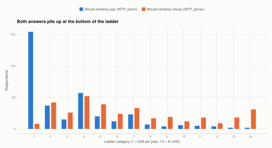
DataFrame(category = 1:14, euros = [EURO_AMOUNT[k] for k in 1:14],
          would_pay = min_counts, would_refuse = max_counts)
14×4 DataFrame
| Row | category | euros | would_pay | would_refuse |
|---|---|---|---|---|
| Int64 | Float64 | Int64 | Int64 | |
| 1 | 1 | 48.0 | 154 | 8 |
| 2 | 2 | 72.0 | 37 | 42 |
| 3 | 3 | 84.0 | 15 | 26 |
| 4 | 4 | 108.0 | 57 | 52 |
| 5 | 5 | 156.0 | 20 | 39 |
| 6 | 6 | 192.0 | 12 | 24 |
| 7 | 7 | 252.0 | 23 | 33 |
| 8 | 8 | 324.0 | 7 | 17 |
| 9 | 9 | 432.0 | 4 | 19 |
| 10 | 10 | 540.0 | 6 | 12 |
| 11 | 11 | 720.0 | 5 | 18 |
| 12 | 12 | 960.0 | 4 | 9 |
| 13 | 13 | 1200.0 | 2 | 18 |
| 14 | 14 | 1440.0 | 2 | 31 |
Both distributions are heavily skewed toward the low categories, and the two are shaped differently in a revealing way. The “would certainly pay” answers concentrate hardest at the very bottom, while the “would certainly refuse” answers sit higher and are more spread out — which is mechanically necessary, since each respondent’s refuse-point is above their pay-point, but the size of the gap is what the design is trying to elicit.
There is visible clustering on particular rungs rather than a smooth decline, which is the signature of a categorical instrument: respondents anchor on round-looking options.
(b) and (c) Average WTP.
survey.WTP_average = [(a === missing || b === missing) ? missing : (a + b) / 2
                      for (a, b) in zip(survey.min_euro, survey.max_euro)]
twpl_wtp = Float64.(collect(skipmissing(survey.WTP_average)))

(respondents = length(twpl_wtp),
 mean = round(mean(twpl_wtp), digits = 2),
 median = round(median(twpl_wtp), digits = 2),
 sd = round(std(twpl_wtp), digits = 2),
 range = extrema(twpl_wtp))
(respondents = 348, mean = 268.53, median = 132.0, sd = 287.71, range = (48.0, 1440.0))Mean €268.53 and median €132.00, both matching the book. The mean is more than double the median, which is the whole story of this variable: a minority naming amounts near the top of the ladder drags the average far above the typical respondent. With €48 to €1,440 available and a median of €132, most people sat on the bottom few rungs.
Of the 506 ladder respondents, 348 produced a usable average — the rest either named no amount, said they would pay zero, or said they would not vote.
(d) What predicts willingness to pay.
survey.female = [(s === missing || s === nothing) ? missing :
                 Float64(lowercase(string(s)) == "female") for s in survey.sex]

wtp_corr = DataFrame(variable = String[], correlation = Float64[], n = Int[])
for col in [:education, :female, :climate, :gov_intervention, :pro_environment]
    ok = .!ismissing.(survey.WTP_average) .& .!ismissing.(survey[!, col])
    push!(wtp_corr, (string(col),
                     round(cor(Float64.(survey[ok, :WTP_average]),
                               Float64.(survey[ok, col])), digits = 8), count(ok)))
end
wtp_corr
5×3 DataFrame
| Row | variable | correlation | n |
|---|---|---|---|
| String | Float64 | Int64 | |
| 1 | education | 0.138174 | 348 |
| 2 | female | -0.0369497 | 348 |
| 3 | climate | -0.144621 | 348 |
| 4 | gov_intervention | -0.188452 | 348 |
| 5 | pro_environment | 0.187503 | 348 |
All five reproduce the published values to eight decimals, with one sign difference explained below.
Every correlation is small — the largest is under 0.19 — so respondent characteristics explain very little of what people said they would pay. Within that, the signs are all interpretable and all point the same way:
- Climate scepticism −0.145. More sceptical respondents would pay less. Recall from Q3 that a high value on this index is scepticism, so the negative sign is the expected direction, not a puzzle.
- Preference for government intervention −0.188, the strongest of the five. The index is coded so that high means less appetite for state action, so people who want government to intervene more would pay more.
- Personal responsibility +0.188. Respondents who feel obliged to act pro-environmentally would pay more.
- Education +0.138. More educated respondents would pay more, which is the usual finding and confounded with income.
- Sex −0.037. Effectively zero.
NoteThe sex correlation’s sign depends on an arbitrary coding choice
The book prints +0.03694972; this gives −0.03694972 — the same magnitude, opposite sign. The variable is text, "female" or "male", so turning it into a number requires picking which one is 1. Coding female as 1 gives the negative value; coding male as 1 gives the book’s.
Neither is wrong, but neither is self-explanatory either, which is the point: a dummy’s sign is meaningless without stating its coding. This page codes female = 1, so the negative correlation reads “women stated slightly lower WTP”.
Q2. The dichotomous-choice demand curve
The DC group each saw one amount and voted. Aggregating across the amounts traces out something that looks like a demand curve.
(a) Votes by amount.
const YES = "support referendum and pay"
const NO = "do not support referendum and no pay"
const ABSTAIN = "would not vote"

dc = group_rows("ref")
amounts = sort(unique(skipmissing(dc.costs)))
votes = DataFrame(euros = Float64[], yes = Int[], no = Int[], abstain = Int[], total = Int[],
                  pct_yes_abstain_as_no = Float64[], pct_yes_abstain_dropped = Float64[])
for a in amounts
    rows = dc[coalesce.(dc.costs .== a, false), :]
    outcome = [string(v) for v in rows.DC_ref_outcome]
    y, n, ab = count(==(YES), outcome), count(==(NO), outcome), count(==(ABSTAIN), outcome)
    push!(votes, (a, y, n, ab, y + n + ab,
                  round(100 * y / (y + n + ab), digits = 2),
                  round(100 * y / (y + n), digits = 2)))
end
votes
14×7 DataFrame
| Row | euros | yes | no | abstain | total | pct_yes_abstain_as_no | pct_yes_abstain_dropped |
|---|---|---|---|---|---|---|---|
| Float64 | Int64 | Int64 | Int64 | Int64 | Float64 | Float64 | |
| 1 | 48.0 | 32 | 21 | 12 | 65 | 49.23 | 60.38 |
| 2 | 72.0 | 40 | 30 | 11 | 81 | 49.38 | 57.14 |
| 3 | 84.0 | 45 | 24 | 12 | 81 | 55.56 | 65.22 |
| 4 | 108.0 | 31 | 35 | 7 | 73 | 42.47 | 46.97 |
| 5 | 156.0 | 40 | 31 | 13 | 84 | 47.62 | 56.34 |
| 6 | 192.0 | 25 | 25 | 11 | 61 | 40.98 | 50.0 |
| 7 | 252.0 | 28 | 32 | 9 | 69 | 40.58 | 46.67 |
| 8 | 324.0 | 27 | 41 | 16 | 84 | 32.14 | 39.71 |
| 9 | 432.0 | 29 | 35 | 11 | 75 | 38.67 | 45.31 |
| 10 | 540.0 | 22 | 31 | 9 | 62 | 35.48 | 41.51 |
| 11 | 720.0 | 13 | 39 | 12 | 64 | 20.31 | 25.0 |
| 12 | 960.0 | 15 | 28 | 14 | 57 | 26.32 | 34.88 |
| 13 | 1200.0 | 21 | 42 | 11 | 74 | 28.38 | 33.33 |
| 14 | 1440.0 | 15 | 42 | 19 | 76 | 19.74 | 26.32 |
(b), (c) and (d) The demand curve, both ways of handling abstentions.
fig = Figure(size = (900, 500))
ax = Axis(fig[1, 1];
          title = "Demand falls with price, and how you count abstentions shifts the level",
          xlabel = "Annual amount offered (€, log scale)",
          ylabel = "Voting yes (%)",
          xscale = log10, xticks = (amounts, string.(Int.(amounts))),
          limits = (nothing, (0, 100)))
for (j, (col, lab)) in enumerate([(:pct_yes_abstain_as_no, "Abstain counted as no"),
                                  (:pct_yes_abstain_dropped, "Abstain excluded")])
    lines!(ax, votes.euros, votes[!, col]; color = series_color(j), linewidth = 2.5)
    scatter!(ax, votes.euros, votes[!, col]; color = series_color(j))
    text!(ax, votes.euros[end], votes[!, col][end]; text = lab, fontsize = 10,
          align = (:right, :top), offset = (-6, -8), color = INK_SECONDARY)
end
fig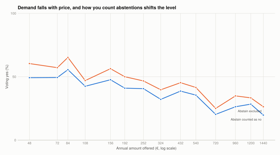
The curve slopes down, which is the basic sanity check — a higher price brings fewer yes votes — and it is worth appreciating that this is not guaranteed in a contingent-valuation survey. Respondents seeing only one amount cannot anchor on the others, so the downward slope is evidence that people responded to the price rather than to the topic.
Two features stand out. The curve is far from a straight line even on a log axis, and the share saying yes does not approach zero at the top amount — a floor of respondents will approve any amount, which is what “protest in the other direction” looks like.
How abstentions are treated shifts the level but not the shape. Counting them as no is the conservative reading: someone who declines to vote has not agreed to pay. Excluding them assumes abstainers would have split like those who voted. The two curves stay roughly parallel, so the qualitative conclusion does not depend on the choice — but the level difference is large enough that a WTP estimate read off this curve would.
The conservative treatment is the defensible default here, because the alternative assumes abstention is unrelated to price, and the table shows abstention is not evenly spread across amounts.
Q3. Does the question format change the answer?
(a) The two formats side by side. For DC respondents, willingness to pay is the amount they were offered and accepted; for ladder respondents it is the average of their two figures.
dc_wtp = Float64[row.costs for row in eachrow(dc)
                 if row.costs !== missing && string(row.DC_ref_outcome) == YES]

comparison = DataFrame(
    format = ["DC", "TWPL"],
    n = [length(dc_wtp), length(twpl_wtp)],
    mean = round.([mean(dc_wtp), mean(twpl_wtp)], digits = 2),
    sd = round.([std(dc_wtp), std(twpl_wtp)], digits = 2),
    median = [median(dc_wtp), median(twpl_wtp)])
comparison
2×5 DataFrame
| Row | format | n | mean | sd | median |
|---|---|---|---|---|---|
| String | Int64 | Float64 | Float64 | Float64 | |
| 1 | DC | 383 | 348.19 | 378.65 | 192.0 |
| 2 | TWPL | 348 | 268.53 | 287.71 | 132.0 |
Every value matches the published table: DC mean €348.19 on 383 respondents, ladder mean €268.53 on 348, with medians of €192 and €132.
(b) A confidence interval for the difference.
test = UnequalVarianceTTest(dc_wtp, twpl_wtp)
lower, upper = confint(test)

DataFrame(quantity = ["Difference in means (DC − TWPL)", "Standard error of the difference",
                      "95% CI lower", "95% CI upper", "95% CI half-width", "p-value"],
          value = round.([mean(dc_wtp) - mean(twpl_wtp),
                          sqrt(var(dc_wtp) / length(dc_wtp) + var(twpl_wtp) / length(twpl_wtp)),
                          lower, upper, (upper - lower) / 2, pvalue(test)], digits = 5))
6×2 DataFrame
| Row | quantity | value |
|---|---|---|
| String | Float64 | |
| 1 | Difference in means (DC − TWPL) | 79.6535 |
| 2 | Standard error of the difference | 24.7429 |
| 3 | 95% CI lower | 31.0752 |
| 4 | 95% CI upper | 128.232 |
| 5 | 95% CI half-width | 48.5783 |
| 6 | p-value | 0.00134 |
WarningThe published interval is a 5% confidence interval, not a 95% one
The book reports the interval as [78.10, 81.21], a half-width of 1.55 on a difference of 79.66, and concludes the difference is “precisely estimated”. Its walk-through shows the call that produced it:
t.test(DC_WTP, TWPL_WTP, conf.level = 0.05)$conf.int
## [1] 78.10141 81.20560
conf.level is the confidence level, so 0.05 requests a 5% interval — one designed to contain the true difference 5% of the time. It looks precise because it is tiny by construction. The intended argument was almost certainly 0.95; 0.05 is the significance level \(\alpha\), which is a natural thing to reach for and the opposite of what this parameter wants.
Reproducing both levels from the same data settles it:
se = sqrt(var(dc_wtp) / length(dc_wtp) + var(twpl_wtp) / length(twpl_wtp))
difference = mean(dc_wtp) - mean(twpl_wtp)
# Welch-Satterthwaite degrees of freedom, as used by both R's t.test and
# HypothesisTests.UnequalVarianceTTest.
df = se^4 / ((var(dc_wtp) / length(dc_wtp))^2 / (length(dc_wtp) - 1) +
             (var(twpl_wtp) / length(twpl_wtp))^2 / (length(twpl_wtp) - 1))

DataFrame(conf_level = [0.95, 0.05],
          multiplier = round.([quantile(TDist(df), (1 + l) / 2) for l in [0.95, 0.05]],
                              digits = 6),
          half_width = round.([quantile(TDist(df), (1 + l) / 2) * se for l in [0.95, 0.05]],
                              digits = 4),
          lower = round.([difference - quantile(TDist(df), (1 + l) / 2) * se
                          for l in [0.95, 0.05]], digits = 4),
          upper = round.([difference + quantile(TDist(df), (1 + l) / 2) * se
                          for l in [0.95, 0.05]], digits = 4))
2×5 DataFrame
| Row | conf_level | multiplier | half_width | lower | upper |
|---|---|---|---|---|---|
| Float64 | Float64 | Float64 | Float64 | Float64 | |
| 1 | 0.95 | 1.96332 | 48.5783 | 31.0752 | 128.232 |
| 2 | 0.05 | 0.062729 | 1.5521 | 78.1014 | 81.2056 |
The 5% row reproduces the book’s printed bounds. The real 95% interval is about 31 times wider: roughly [31, 128] against [78.1, 81.2].
Julia will not make this mistake quietly. confint(test; level = 0.05) throws coverage level 0.05 not in range (0.5, 1) — the API rejects a coverage below one half as incoherent, where R’s t.test accepts it and returns an interval. That is a case where the stricter interface is worth the inflexibility.
The direction of the conclusion survives. The correct interval still excludes zero comfortably, so DC really does produce higher stated WTP. What does not survive is the claim that the difference is precisely estimated, or that “the confidence interval lower bound is a long way from 0” in the sense the book means — the lower bound is €31, not €78, and the difference could plausibly be anywhere from a third of the ladder mean to half again as much.
(c) Medians against means.
DataFrame(measure = ["Mean", "Median"],
          DC = [comparison.mean[1], comparison.median[1]],
          TWPL = [comparison.mean[2], comparison.median[2]],
          difference = [comparison.mean[1] - comparison.mean[2],
                        comparison.median[1] - comparison.median[2]],
          ratio = round.([comparison.mean[1] / comparison.mean[2],
                          comparison.median[1] / comparison.median[2]], digits = 3))
2×5 DataFrame
| Row | measure | DC | TWPL | difference | ratio |
|---|---|---|---|---|---|
| String | Float64 | Float64 | Float64 | Float64 | |
| 1 | Mean | 348.19 | 268.53 | 79.66 | 1.297 |
| 2 | Median | 192.0 | 132.0 | 60.0 | 1.455 |
The mean moves by €79.66 and the median by €60 — but as a proportion the median is the less stable of the two here: 1.45 times against 1.30 for the mean. That is worth stating plainly because the book concludes the opposite, that “the median is therefore more robust to changes in the question format”.
On these numbers the median is not more robust in relative terms. What is true is the related point the book is reaching for: the median is far less sensitive to the top of the distribution, which is why the DC mean sits at €348 against a median of €192.
(d) Which should a government use? The honest answer depends on the question being asked, and the two measures answer different ones.
- The mean is what a budget needs. Total revenue from a charge is the mean times the number of payers, so if the policy question is “does this fund the abatement”, the mean is the relevant statistic. Its weakness is that it is set by the upper tail — a handful of people naming €1,440 move it a long way, and those are exactly the responses most exposed to the hypothetical bias from Q1.
- The median is what a vote needs. A referendum at price \(p\) passes if more than half the electorate would accept \(p\), which is the median WTP by definition. It ignores intensity entirely: someone willing to pay the top ladder amount counts exactly the same as someone a single euro above the median.
Given that the format changes the mean by €80 and neither format’s mean can be checked against behaviour, reporting both and the interval around the difference is the defensible course, which is what this page does and what the mislabelled interval obscured.
What this project covered
| Concept | Where | In Julia |
|---|---|---|
| Reading strict OOXML | Setup | XLSX.readxlsx(path)[sheet][:], not readtable |
Blanks that arrive as nothing |
Setup | handle nothing and missing in the coercion |
| Reverse-coding a Likert item | Q11.1 Q2 | 6 .- x on a 1–5 scale |
| Mapping categories to amounts | Q11.1 Q2 | Dict lookup with get(..., missing) |
| Row means across chosen columns | Q11.1 Q3 | comprehension over eachrow |
| Cronbach’s alpha | Q11.1 Q4 | cronbach_alpha(items) from the shared helpers |
| Composition tables by group | Q11.1 Q5 | shares of each group’s non-missing responses |
| Dummy from a text column | Q11.2 Q1 | state the coding — the sign depends on it |
| Log axis with named ticks | Q11.2 Q2 | xscale = log10, xticks = (amounts, labels) |
| Difference in means with a CI | Q11.2 Q3 | UnequalVarianceTTest, confint |
| Welch degrees of freedom | Q11.2 Q3 | Welch–Satterthwaite, then quantile(TDist(df), p) |
| A coverage level below ½ | Q11.2 Q3 | Julia throws; R’s t.test accepts it |
The R → Julia page has the full translation table.