Doing Economics in Julia
  • Home
  • Setup
  • R → Julia
  1. Empirical projects
  2. Extra 2. Carbon taxation
  • Getting started
    • Overview
    • Setup
  • Empirical projects
    • 1. Measuring climate change
    • 2. Data from experiments
    • 3. Measuring a sugar tax
    • 4. Measuring wellbeing
    • 5. Measuring inequality
    • 6. Management practices
    • 7. Supply and demand
    • 8. Cost of unemployment
    • 9. Credit-excluded households
    • 10. Banking systems
    • 11. Willingness to pay
    • 12. Hong Kong cash handout
    • Extra 2. Carbon taxation
  • Reference
    • R → Julia
    • Technical reference

On this page

  • Part 1 — Measuring and explaining support for carbon taxation
    • Q1. How the question was asked
    • Q2. Sample sizes
    • Q3. How the authors recode support, and what it costs
    • Q4 and Q5. The dummy variables
    • Q6 to Q10. Baseline support, in the control group only
    • Q11 and Q12. Who supports it
  • Part 2 — Explaining rural backlashes
    • Q1 to Q3. The correlation among rural respondents
    • Q4 to Q6. The information experiment
    • What this establishes, and what it does not
    • What this project covered
  • View source
  • Report an issue
  1. Empirical projects
  2. Extra 2. Carbon taxation

Extra 2. The politics of carbon taxation

Why rural voters reject carbon taxes, and a survey experiment that moves the belief

A UK survey of 2,997 respondents on carbon taxation, from Hope, Limberg and Steinebach (2026). It is a survey experiment: half the sample received an information treatment before being asked their views, so the difference between the halves is caused by the information rather than merely correlated with it.

The argument being tested is that rural opposition to carbon taxes is not only about the higher costs rural households face, but about fairness — a sense that the state already treats these communities unequally, and that a carbon tax adds to the injury.

  • Part 1 — measuring and explaining support for carbon taxation
  • Part 2 — explaining rural backlashes

Concepts: Likert scales, dummy variables, conditional means, and an information-provision survey experiment as a way to test a causal claim about beliefs. Book pages: project, R walk-through, solutions.

using XLSX, DataFrames
using Statistics
using HypothesisTests
using CairoMakie
using DoingEconomics

CairoMakie.activate!(type = "svg")
use_doingecon_theme!()
path = rawpath("14", "carbon-tax-hope.xlsx")

function sheet_frame(p, name)
    cells = XLSX.readxlsx(p)[name][:]
    return DataFrame([cells[2:end, j] for j in axes(cells, 2)],
                     Symbol.(string.(cells[1, :])); makeunique = true)
end

survey = sheet_frame(path, "Data")

function num(x)
    (x === missing || x === nothing) && return missing
    x isa Number && return Float64(x)
    parsed = tryparse(Float64, string(x))
    return parsed === nothing ? missing : parsed
end
for col in [:age, :treatment, :carbon_tax_support, :unequal_treatment, :carbon_tax_unfairness]
    survey[!, col] = num.(survey[!, col])
end
text_col(v) = [x === missing || x === nothing ? missing : string(x) for x in v]
for col in [:neighbourhood, :commute, :partisanship]
    survey[!, col] = text_col(survey[!, col])
end

(respondents = nrow(survey), variables = names(survey))
(respondents = 2997, variables = ["respondent_id", "age", "neighbourhood", "commute", "partisanship", "treatment", "carbon_tax_support", "unequal_treatment", "carbon_tax_unfairness"])

Part 1 — Measuring and explaining support for carbon taxation

Q1. How the question was asked

Both groups are given a short explanation of a carbon tax immediately before being asked their view: how the tax works, that heavier fossil-fuel users pay more, and that it is aimed at climate change.

That explanation is the step taken to improve accuracy. Asking about an unfamiliar policy otherwise measures whatever the respondent imagines the words mean, and “carbon tax” is a phrase many people hold an opinion about without holding a definition. Briefing everyone identically means the answers refer to the same object — and because both arms get it, it is not the experimental treatment.

Q2. Sample sizes

DataFrame(group = ["Treatment", "Control", "Total"],
          respondents = [count(==(1.0), survey.treatment),
                         count(==(0.0), survey.treatment), nrow(survey)])
3×2 DataFrame
Row group respondents
String Int64
1 Treatment 1481
2 Control 1516
3 Total 2997

2,997 respondents, 1,481 treated and 1,516 control, all three matching the published solution. The split is near-even, as random assignment should produce.

Q3. How the authors recode support, and what it costs

ImportantThe book’s own description of the scale is inverted

The project text says support is measured “on a 5-point scale running from 1 for ‘strongly oppose’ to 5 for ‘strongly support’”. The data dictionary in the spreadsheet says the opposite: 1 is strongly support and 5 is strongly oppose.

The dictionary is right, and the book’s own instructions confirm it — the dummy variable is defined as 1 when carbon_tax_support is 1 or 2, described as “strongly support or support”. That only makes sense if low numbers mean support.

Taking the question text at face value would invert every result on this page while leaving all the arithmetic looking perfectly reasonable. The check is the published frequency table, which this page reproduces below: if the coding were reversed, the counts would attach to the opposite labels.

The authors collapse the five-point scale to a dummy: 1 for support or strong support, 0 otherwise.

  • The advantage is interpretability. The mean of a 0/1 variable is the share supporting, so every conditional mean below reads directly as a percentage, and it behaves well in a regression.
  • The cost is intensity. Someone who strongly supports and someone who merely supports become identical, as do a neutral respondent and a strong opponent. The variable can no longer detect a change that moves people from “oppose” to “strongly oppose” — a real hardening of opinion that this measure records as nothing at all.

Q4 and Q5. The dummy variables

# Missing stays missing throughout: a respondent who skipped the question is not a zero.
survey.supports = [s === missing ? missing : Float64(s <= 2) for s in survey.carbon_tax_support]
survey.aged_40_plus = [a === missing ? missing : Float64(a >= 40) for a in survey.age]
survey.commutes_by_car = [c === missing ? missing : Float64(c == "Car") for c in survey.commute]
survey.rural = [n === missing ? missing : Float64(n == "Rural") for n in survey.neighbourhood]
survey.high_unequal = [u === missing ? missing : Float64(u >= 8)
                       for u in survey.unequal_treatment]

const DUMMIES = [:supports, :aged_40_plus, :commutes_by_car, :rural, :high_unequal]
DataFrame(dummy = DUMMIES,
          ones = [count(==(1.0), skipmissing(survey[!, d])) for d in DUMMIES],
          zeros = [count(==(0.0), skipmissing(survey[!, d])) for d in DUMMIES],
          missing_n = [count(ismissing, survey[!, d]) for d in DUMMIES],
          mean = [round(mean(skipmissing(survey[!, d])), digits = 4) for d in DUMMIES])
5×5 DataFrame
Row dummy ones zeros missing_n mean
Symbol Int64 Int64 Int64 Float64
1 supports 1318 1623 56 0.4481
2 aged_40_plus 1735 1064 198 0.6199
3 commutes_by_car 1124 917 956 0.5507
4 rural 613 2384 0 0.2045
5 high_unequal 1727 1270 0 0.5762

Keeping missing as missing matters more than it looks. Coding a non-response as 0 would silently recruit every respondent who skipped the question into the “does not support” camp, which is a different claim from “did not say”.

Q6 to Q10. Baseline support, in the control group only

Everything from here to the end of Part 1 uses the control group, so it measures support uncontaminated by the experimental treatment.

control = survey[survey.treatment .== 0.0, :]
const SCALE = [1 => "Strongly support", 2 => "Support", 3 => "Neither support nor oppose",
               4 => "Oppose", 5 => "Strongly oppose"]
answered = count(!ismissing, control.carbon_tax_support)

distribution = DataFrame(
    code = first.(SCALE),
    response = last.(SCALE),
    respondents = [count(==(Float64(k)), skipmissing(control.carbon_tax_support))
                   for k in first.(SCALE)])
distribution.percentage = round.(100 .* distribution.respondents ./ answered, digits = 1)
distribution
5×4 DataFrame
Row code response respondents percentage
Int64 String Int64 Float64
1 1 Strongly support 131 8.8
2 2 Support 557 37.3
3 3 Neither support nor oppose 282 18.9
4 4 Oppose 317 21.2
5 5 Strongly oppose 207 13.9
Table 1: Distribution of carbon tax support in the control group. Reproduces the book’s Solution figure 1.
(control_group = nrow(control), answered = answered,
 did_not_answer = nrow(control) - answered)
(control_group = 1516, answered = 1494, did_not_answer = 22)

All five counts and all five percentages match the published table. Note that 22 of the 1,516 control respondents did not answer, so the percentages are shares of 1,494.

ordered = reverse(distribution)

fig = Figure(size = (820, 480))
ax = Axis(fig[1, 1];
          title = "Support outweighs opposition, but a third of the public is opposed",
          ylabel = "% of respondents",
          xticks = (1:5, ordered.response), xticklabelrotation = pi / 9,
          limits = (nothing, (0, 44)))
barplot!(ax, 1:5, ordered.percentage; width = 0.6, color = series_color(1))
for (x, v) in zip(1:5, ordered.percentage)
    text!(ax, x, v; text = string(v) * "%", fontsize = 11,
          align = (:center, :bottom), offset = (0, 4), color = INK)
end
fig
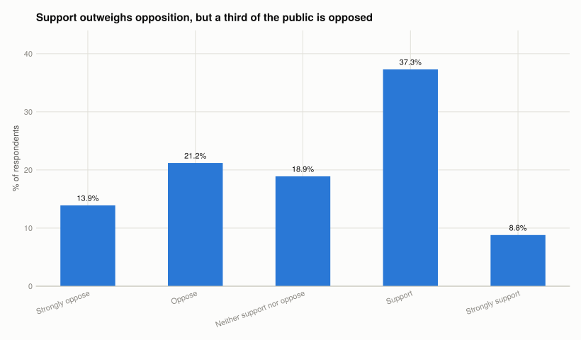
Figure 1: Percentage of control-group respondents at each level of carbon tax support, ordered from strongest opposition to strongest support so the axis reads left to right as increasing support. One series, so one colour; every bar is labelled, which is what the book’s question asks for.

The modal answer is “Support”, at 37.3%, and only 8.8% strongly support. Adding the two support categories gives 46.1%; the two opposition categories give 35.1%; 18.9% sit in the middle.

(support_share = round(mean(skipmissing(control.supports)), digits = 4),
 from_the_table = round((distribution.percentage[1] + distribution.percentage[2]) / 100,
                        digits = 4))
(support_share = 0.4605, from_the_table = 0.461)

The dummy’s mean is 0.461, which is exactly the combined “support” plus “strongly support” share from the table — matching the published value. That identity is the whole reason the dummy is convenient: its average is the share.

So is carbon taxation popular in the UK? More people support it than oppose it, by about 11 percentage points. But two features of the distribution matter more than the sign:

  • Support is broad and shallow, opposition is narrower and deeper. Only 8.8% strongly support, while 13.9% strongly oppose. The intense minority is on the opposing side, and intensity is what turns opinion into protest — which is what Part 2 is about.
  • A third of the public is against it, and 18.9% more are uncommitted. A policy with 46% support is not one a government can treat as settled.

Q11 and Q12. Who supports it

function conditional(col, labels)
    out = DataFrame(group = String[], respondents = Int[], support = Float64[])
    for (v, label) in labels
        sub = control[coalesce.(control[!, col] .== v, false), :]
        s = collect(skipmissing(sub.supports))
        push!(out, (label, length(s), round(mean(s), digits = 4)))
    end
    return out
end

vcat(conditional(:aged_40_plus, [0.0 => "Under 40", 1.0 => "40 and over"]),
     conditional(:commutes_by_car, [0.0 => "Does not commute by car",
                                    1.0 => "Commutes by car"]),
     conditional(:rural, [0.0 => "Non-rural", 1.0 => "Rural"]),
     conditional(:high_unequal, [0.0 => "Perceives less unequal treatment (0–7)",
                                 1.0 => "Perceives unequal treatment (8–10)"]))
8×3 DataFrame
Row group respondents support
String Int64 Float64
1 Under 40 528 0.5303
2 40 and over 867 0.4141
3 Does not commute by car 451 0.5521
4 Commutes by car 562 0.4075
5 Non-rural 1174 0.4685
6 Rural 320 0.4312
7 Perceives less unequal treatment (0–7) 683 0.4949
8 Perceives unequal treatment (8–10) 811 0.4316
Table 2: Share supporting a carbon tax within each subgroup of the control group. Reproduces the book’s Solution figures 3 to 6.
parties = DataFrame(party = String[], respondents = Int[], support = Float64[])
small = Float64[]
for p in sort(unique(skipmissing(control.partisanship)))
    s = collect(skipmissing(control[coalesce.(control.partisanship .== p, false), :supports]))
    if length(s) < 20
        append!(small, s)
    else
        push!(parties, (p, length(s), round(mean(s), digits = 4)))
    end
end
isempty(small) || push!(parties, ("Smaller parties (combined)", length(small),
                                  round(mean(small), digits = 4)))
sort!(parties, :support, rev = true)
parties
9×3 DataFrame
Row party respondents support
String Int64 Float64
1 Green Party of England and Wales 142 0.6901
2 Scottish National Party 47 0.617
3 Labour Party 500 0.552
4 Liberal Democrats 140 0.5286
5 Other 44 0.5
6 Smaller parties (combined) 18 0.4444
7 Conservative Party 265 0.3434
8 Prefer not to say 42 0.2619
9 Reform UK 108 0.1667
Table 3: Share supporting a carbon tax by party, control group. Parties with fewer than 20 respondents are grouped as “Smaller parties” rather than reported separately, since a share computed on six people carries no information.

Party is by far the strongest divide. Green voters support at 0.69 and Reform UK voters at 0.17 — a four-fold gap, and wider than anything else in the data. Labour (0.55), Liberal Democrat (0.53) and SNP (0.62) sit above the average; Conservative (0.34) below.

The demographic splits are real but much smaller:

  • Age: under-40s 0.53 against 0.41 for those 40 and over — a 12-point gap.
  • Car commuting: 0.55 for non-car commuters against 0.41 for car commuters. This is the cost channel in its most direct form: a carbon tax raises the price of fuel, and people who drive to work pay it.
  • Rural: 0.43 against 0.47 non-rural — only about 4 points, which is the surprise.

That small rural gap is the puzzle Part 2 exists to explain. Rural residents are the group whose backlash the article is about, and on this measure they are barely less supportive than everyone else. Whatever drives rural opposition is not visible as a large average difference — it needs the mechanism, not the headline.

The last row points at it. Respondents who feel the state treats people unequally support at 0.43 against 0.49 for those who do not — a gap comparable to the rural gap, on a variable that is not about geography at all.

Two variables absent from this dataset that should matter:

  1. Income. A carbon tax is regressive relative to income, so willingness to pay for it should fall as income falls. Its absence is the biggest gap here, and it is likely correlated with several variables that are present, including car commuting.
  2. Home heating type. A household on oil or LPG — common in rural areas off the gas grid — faces a much larger bill from a carbon tax than one on mains gas or a heat pump, and unlike commuting it cannot be changed cheaply.

Either could account for part of what the party and commuting variables are currently absorbing.

Part 2 — Explaining rural backlashes

The argument is that rural opposition runs through perceived unfairness: rural communities believe the state already treats them unequally, and read a carbon tax as more of the same.

unequal_treatment measures agreement that the government treats people equally regardless of where they live, reverse-coded so that high values mean perceiving more unequal treatment. carbon_tax_unfairness measures agreement that a carbon tax is unfair because it falls on people the government has already disadvantaged.

Q1 to Q3. The correlation among rural respondents

rural_control = control[coalesce.(control.rural .== 1.0, false), :]

rural_table = DataFrame(perception = ["Low unequal treatment (0–7)",
                                      "High unequal treatment (8–10)"])
for (col, label) in [(:carbon_tax_unfairness, "mean_unfairness"),
                     (:supports, "mean_support")]
    rural_table[!, label] = [
        round(mean(skipmissing(rural_control[coalesce.(rural_control.high_unequal .== v, false),
                                             col])), digits = 4) for v in [0.0, 1.0]]
end
rural_table.respondents = [count(==(v), skipmissing(rural_control.high_unequal))
                           for v in [0.0, 1.0]]
rural_table
2×4 DataFrame
Row perception mean_unfairness mean_support respondents
String Float64 Float64 Int64
1 Low unequal treatment (0–7) 5.127 0.472 126
2 High unequal treatment (8–10) 6.203 0.4051 197
Table 4: Rural control-group respondents split by whether they perceive unequal treatment. Reproduces the book’s Solution figures 7 and 8.

Both published figures reproduce: unfairness 5.1 against 6.2, support 0.47 against 0.41.

ok = .!ismissing.(rural_control.unequal_treatment) .&
     .!ismissing.(rural_control.carbon_tax_unfairness)
(rural_control_respondents = nrow(rural_control),
 correlation = round(cor(Float64.(rural_control[ok, :unequal_treatment]),
                         Float64.(rural_control[ok, :carbon_tax_unfairness])), digits = 4),
 n = count(ok))
(rural_control_respondents = 323, correlation = 0.2029, n = 323)

Among rural control respondents, perceiving unequal treatment goes with both finding the tax unfair and opposing it. The unfairness gap is 1.08 points on an 11-point scale; the support gap is 6.7 percentage points.

The correlation between the two continuous measures is 0.20 — positive and clearly present, but modest. That is worth stating plainly, because it is the honest version of the article’s claim: unequal-treatment perceptions are one input into fairness judgements about carbon taxes, not the dominant one.

And none of this is causal. Both variables are attitudes recorded in the same interview from the same person. A respondent generally aggrieved with government would score high on both without either causing the other. That is precisely what the experiment is for.

Q4 to Q6. The information experiment

The treatment provides information about how the state treats different areas. If the article’s mechanism is right, that information should raise perceived unequal treatment, raise perceived unfairness of the tax, and lower support — among rural respondents.

rural_all = survey[coalesce.(survey.rural .== 1.0, false), :]

effects = DataFrame(outcome = String[], treated = Float64[], n_treated = Int[],
                    control = Float64[], n_control = Int[], difference = Float64[],
                    lower = Float64[], upper = Float64[], p_value = Float64[])
for (col, label) in [(:unequal_treatment, "Unequal treatment perception (0–10)"),
                     (:carbon_tax_unfairness, "Carbon tax unfairness (0–10)"),
                     (:supports, "Supports a carbon tax (0/1)")]
    t = Float64.(collect(skipmissing(rural_all[rural_all.treatment .== 1.0, col])))
    c = Float64.(collect(skipmissing(rural_all[rural_all.treatment .== 0.0, col])))
    test = UnequalVarianceTTest(t, c)
    lo, hi = confint(test)
    push!(effects, (label, round(mean(t), digits = 4), length(t),
                    round(mean(c), digits = 4), length(c),
                    round(mean(t) - mean(c), digits = 4),
                    round(lo, digits = 4), round(hi, digits = 4),
                    round(pvalue(test), digits = 4)))
end
effects
3×9 DataFrame
Row outcome treated n_treated control n_control difference lower upper p_value
String Float64 Int64 Float64 Int64 Float64 Float64 Float64 Float64
1 Unequal treatment perception (0–10) 8.0483 290 7.6904 323 0.3579 0.0487 0.667 0.0234
2 Carbon tax unfairness (0–10) 6.1276 290 5.7833 323 0.3443 -0.0438 0.7324 0.082
3 Supports a carbon tax (0/1) 0.3169 284 0.4312 320 -0.1143 -0.1913 -0.0374 0.0036
Table 5: Treatment against control among rural respondents, with 95% confidence intervals for the difference. Reproduces the p-values in the book’s solutions to Question 6.

All three p-values match the published solutions: 0.023, 0.082 and 0.004.

fig = Figure(size = (960, 420))
for (k, (col, label, limits)) in enumerate([
        (:unequal_treatment, "Unequal treatment\nperception (0–10)", (7.0, 8.6)),
        (:carbon_tax_unfairness, "Carbon tax\nunfairness (0–10)", (5.2, 6.7)),
        (:supports, "Supports a\ncarbon tax", (0.25, 0.50))])
    ax = Axis(fig[1, k]; title = label, titlesize = 12,
              xticks = (1:2, ["Control", "Treatment"]), limits = (nothing, limits))
    for (j, arm) in enumerate([0.0, 1.0])
        v = Float64.(collect(skipmissing(rural_all[rural_all.treatment .== arm, col])))
        half = 1.96 * std(v) / sqrt(length(v))
        barplot!(ax, [j], [mean(v)]; width = 0.45, color = series_color(j),
                 label = j == 1 ? "Control" : "Treatment")
        errorbars!(ax, [j], [mean(v)], [half];
                   color = INK_SECONDARY, whiskerwidth = 12, linewidth = 2)
    end
end
Legend(fig[0, 1:3], fig.content[1]; orientation = :horizontal, framevisible = false)
fig
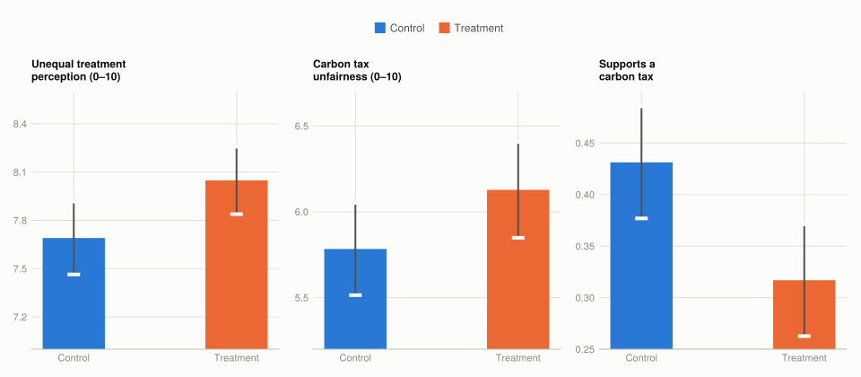
Figure 2: Rural respondents’ mean outcome by experimental arm, with 95% confidence intervals on each group mean. Two series, so the arm carries the colour. Three panels because the outcomes are on different scales — two 0–10 attitude scales and one 0/1 share — and a shared axis would be meaningless.

The experiment supports the mechanism, and the ordering of the three results is the interesting part.

  • Unequal treatment perception rises by 0.36 points [0.05, 0.67], p = 0.023. The information did what it was meant to do: it changed the belief the article says is upstream of everything else.
  • Carbon tax unfairness rises by 0.34 points [−0.04, 0.73], p = 0.082. Same direction, similar size, but the interval includes zero. On a conventional 5% threshold this is not significant, and it is the middle link in the causal chain.
  • Support falls by 11.4 percentage points [−0.19, −0.04], p = 0.004. The largest and most precisely estimated of the three.

Why the middle link being weakest is awkward for the mechanism. The proposed chain runs information → unequal-treatment perception → unfairness perception → lower support. The two ends move clearly and the middle does not quite. If unfairness were the channel carrying the effect through to support, it should be at least as well identified as the outcome it explains.

Two readings, and this design cannot separate them:

  1. The chain holds and the unfairness measure is noisy. An 11-point agree/disagree scale is a coarse instrument for a specific belief, and measurement error attenuates exactly this kind of intermediate estimate. Its point estimate is the right sign and a comparable size.
  2. Information affects support through some other route — general grievance with government, or simply priming a rural identity — and unfairness is a correlate rather than the conduit.

Distinguishing them needs a design that manipulates unfairness perceptions directly, or a formal mediation analysis with its own assumptions. What the experiment does establish is the part that matters most for the article’s headline: telling rural respondents about unequal treatment causes them to withdraw support for a carbon tax.

What this establishes, and what it does not

Established. Rural support for carbon taxation is causally sensitive to beliefs about how the state treats rural areas. An 11-point fall from a short information treatment is a large effect for a survey experiment, and it is not explicable by rural respondents differing from urban ones in some fixed way, because the comparison is within rural respondents randomly assigned.

Not established. Three limits worth being explicit about:

  • Survey responses are not votes or protests. The Gilets Jaunes did not fill in a Likert scale. Whether a stated 11-point shift corresponds to political behaviour is outside this design.
  • The treatment is information a researcher chose to provide. Its effect size depends on that content, and it says how malleable the belief is, not how much of real-world rural opposition the belief currently explains.
  • Durability is unknown. The outcome is measured minutes after the treatment. Attitude effects from information provision are known to decay.

What it implies for policy, taking Part 1 together with Part 2: the rural support gap is small on average (about 4 points) but highly responsive to fairness framing. A carbon tax introduced without visible attention to distribution across places has a latent constituency against it that can be activated by a single piece of information. Revenue recycling targeted at the places that pay most is the obvious lever, and it is aimed at exactly the belief this experiment shows is doing the work.

What this project covered

Concept Where In Julia
A scale coded opposite to its description Q1 Q3 check counts against the published table
Dummy variables preserving missing Q1 Q4 s === missing ? missing : Float64(s <= 2)
The mean of a dummy as a share Q1 Q10 mean(skipmissing(col))
Conditional means by subgroup Q1 Q11 mask, skipmissing, mean
Suppressing tiny subgroups Q1 Q11 pool categories under 20 respondents
Treatment vs control difference Q2 Q6 UnequalVarianceTTest, confint, pvalue
Error bars on group means Q2 Q6 errorbars! with 1.96 * sem
Panels for different scales Q2 Q6 one Axis per outcome, own limits
Reversing a table for display Q1 Q8 reverse(df)

The R → Julia page has the full translation table.

12. Hong Kong cash handout
R → Julia
Source Code
---
title: "Extra 2. The politics of carbon taxation"
subtitle: "Why rural voters reject carbon taxes, and a survey experiment that moves the belief"
engine: julia
julia:
  exeflags: ["--project=@."]
---

A UK survey of 2,997 respondents on carbon taxation, from Hope, Limberg and Steinebach (2026).
It is a **survey experiment**: half the sample received an information treatment before being
asked their views, so the difference between the halves is caused by the information rather than
merely correlated with it.

The argument being tested is that rural opposition to carbon taxes is not only about the higher
costs rural households face, but about **fairness** — a sense that the state already treats
these communities unequally, and that a carbon tax adds to the injury.

- **[Part 1](#part-1)** — measuring and explaining support for carbon taxation
- **[Part 2](#part-2)** — explaining rural backlashes

Concepts: **Likert scales**, **dummy variables**, **conditional means**, and an
**information-provision survey experiment** as a way to test a causal claim about beliefs. Book
pages: [project](https://books.core-econ.org/doing-economics/book/text/14-01.html),
[R walk-through](https://books.core-econ.org/doing-economics/book/text/14-03.html),
[solutions](https://books.core-econ.org/doing-economics/book/text/14-06.html).

```{julia}
#| label: setup
#| output: false
using XLSX, DataFrames
using Statistics
using HypothesisTests
using CairoMakie
using DoingEconomics

CairoMakie.activate!(type = "svg")
use_doingecon_theme!()
```

```{julia}
#| label: read-survey
path = rawpath("14", "carbon-tax-hope.xlsx")

function sheet_frame(p, name)
    cells = XLSX.readxlsx(p)[name][:]
    return DataFrame([cells[2:end, j] for j in axes(cells, 2)],
                     Symbol.(string.(cells[1, :])); makeunique = true)
end

survey = sheet_frame(path, "Data")

function num(x)
    (x === missing || x === nothing) && return missing
    x isa Number && return Float64(x)
    parsed = tryparse(Float64, string(x))
    return parsed === nothing ? missing : parsed
end
for col in [:age, :treatment, :carbon_tax_support, :unequal_treatment, :carbon_tax_unfairness]
    survey[!, col] = num.(survey[!, col])
end
text_col(v) = [x === missing || x === nothing ? missing : string(x) for x in v]
for col in [:neighbourhood, :commute, :partisanship]
    survey[!, col] = text_col(survey[!, col])
end

(respondents = nrow(survey), variables = names(survey))
```

# Part 1 — Measuring and explaining support for carbon taxation {#part-1}

## Q1. How the question was asked {#p1-q1}

Both groups are given a short explanation of a carbon tax immediately before being asked their
view: how the tax works, that heavier fossil-fuel users pay more, and that it is aimed at
climate change.

**That explanation is the step taken to improve accuracy.** Asking about an unfamiliar policy
otherwise measures whatever the respondent imagines the words mean, and "carbon tax" is a phrase
many people hold an opinion about without holding a definition. Briefing everyone identically
means the answers refer to the same object — and because *both* arms get it, it is not the
experimental treatment.

## Q2. Sample sizes {#p1-q2}

```{julia}
#| label: sample-sizes
DataFrame(group = ["Treatment", "Control", "Total"],
          respondents = [count(==(1.0), survey.treatment),
                         count(==(0.0), survey.treatment), nrow(survey)])
```

**2,997 respondents, 1,481 treated and 1,516 control**, all three matching the published
solution. The split is near-even, as random assignment should produce.

## Q3. How the authors recode support, and what it costs {#p1-q3}

::: {.callout-important}
## The book's own description of the scale is inverted

The project text says support is measured "on a 5-point scale running from 1 for 'strongly
oppose' to 5 for 'strongly support'". The **data dictionary in the spreadsheet says the
opposite**: 1 is strongly support and 5 is strongly oppose.

The dictionary is right, and the book's own instructions confirm it — the dummy variable is
defined as 1 when `carbon_tax_support` is 1 or 2, described as "strongly support or support".
That only makes sense if low numbers mean support.

Taking the question text at face value would invert every result on this page while leaving all
the arithmetic looking perfectly reasonable. The check is the published frequency table, which
this page reproduces below: if the coding were reversed, the counts would attach to the opposite
labels.
:::

The authors collapse the five-point scale to a **dummy**: 1 for support or strong support, 0
otherwise.

- **The advantage is interpretability.** The mean of a 0/1 variable *is* the share supporting, so
  every conditional mean below reads directly as a percentage, and it behaves well in a
  regression.
- **The cost is intensity.** Someone who strongly supports and someone who merely supports become
  identical, as do a neutral respondent and a strong opponent. The variable can no longer detect
  a change that moves people from "oppose" to "strongly oppose" — a real hardening of opinion
  that this measure records as nothing at all.

## Q4 and Q5. The dummy variables {#p1-q4}

```{julia}
#| label: dummies
# Missing stays missing throughout: a respondent who skipped the question is not a zero.
survey.supports = [s === missing ? missing : Float64(s <= 2) for s in survey.carbon_tax_support]
survey.aged_40_plus = [a === missing ? missing : Float64(a >= 40) for a in survey.age]
survey.commutes_by_car = [c === missing ? missing : Float64(c == "Car") for c in survey.commute]
survey.rural = [n === missing ? missing : Float64(n == "Rural") for n in survey.neighbourhood]
survey.high_unequal = [u === missing ? missing : Float64(u >= 8)
                       for u in survey.unequal_treatment]

const DUMMIES = [:supports, :aged_40_plus, :commutes_by_car, :rural, :high_unequal]
DataFrame(dummy = DUMMIES,
          ones = [count(==(1.0), skipmissing(survey[!, d])) for d in DUMMIES],
          zeros = [count(==(0.0), skipmissing(survey[!, d])) for d in DUMMIES],
          missing_n = [count(ismissing, survey[!, d]) for d in DUMMIES],
          mean = [round(mean(skipmissing(survey[!, d])), digits = 4) for d in DUMMIES])
```

Keeping missing as missing matters more than it looks. Coding a non-response as 0 would silently
recruit every respondent who skipped the question into the "does not support" camp, which is a
different claim from "did not say".

## Q6 to Q10. Baseline support, in the control group only {#p1-q7}

Everything from here to the end of Part 1 uses the **control group**, so it measures support
uncontaminated by the experimental treatment.

```{julia}
#| label: tbl-distribution
#| tbl-cap: "Distribution of carbon tax support in the control group. Reproduces the book's Solution figure 1."
control = survey[survey.treatment .== 0.0, :]
const SCALE = [1 => "Strongly support", 2 => "Support", 3 => "Neither support nor oppose",
               4 => "Oppose", 5 => "Strongly oppose"]
answered = count(!ismissing, control.carbon_tax_support)

distribution = DataFrame(
    code = first.(SCALE),
    response = last.(SCALE),
    respondents = [count(==(Float64(k)), skipmissing(control.carbon_tax_support))
                   for k in first.(SCALE)])
distribution.percentage = round.(100 .* distribution.respondents ./ answered, digits = 1)
distribution
```

```{julia}
#| label: coverage
(control_group = nrow(control), answered = answered,
 did_not_answer = nrow(control) - answered)
```

All five counts and all five percentages match the published table. Note that **22 of the 1,516
control respondents did not answer**, so the percentages are shares of 1,494.

```{julia}
#| label: fig-distribution
#| fig-cap: "Percentage of control-group respondents at each level of carbon tax support, ordered from strongest opposition to strongest support so the axis reads left to right as increasing support. One series, so one colour; every bar is labelled, which is what the book's question asks for."
ordered = reverse(distribution)

fig = Figure(size = (820, 480))
ax = Axis(fig[1, 1];
          title = "Support outweighs opposition, but a third of the public is opposed",
          ylabel = "% of respondents",
          xticks = (1:5, ordered.response), xticklabelrotation = pi / 9,
          limits = (nothing, (0, 44)))
barplot!(ax, 1:5, ordered.percentage; width = 0.6, color = series_color(1))
for (x, v) in zip(1:5, ordered.percentage)
    text!(ax, x, v; text = string(v) * "%", fontsize = 11,
          align = (:center, :bottom), offset = (0, 4), color = INK)
end
fig
```

**The modal answer is "Support", at 37.3%**, and only 8.8% strongly support. Adding the two
support categories gives **46.1%**; the two opposition categories give **35.1%**; 18.9% sit in
the middle.

```{julia}
#| label: dummy-mean
(support_share = round(mean(skipmissing(control.supports)), digits = 4),
 from_the_table = round((distribution.percentage[1] + distribution.percentage[2]) / 100,
                        digits = 4))
```

**The dummy's mean is 0.461**, which is exactly the combined "support" plus "strongly support"
share from the table — matching the published value. That identity is the whole reason the dummy
is convenient: its average *is* the share.

**So is carbon taxation popular in the UK?** More people support it than oppose it, by about 11
percentage points. But two features of the distribution matter more than the sign:

- **Support is broad and shallow, opposition is narrower and deeper.** Only 8.8% strongly
  support, while 13.9% strongly oppose. The intense minority is on the opposing side, and
  intensity is what turns opinion into protest — which is what Part 2 is about.
- **A third of the public is against it**, and 18.9% more are uncommitted. A policy with 46%
  support is not one a government can treat as settled.

## Q11 and Q12. Who supports it {#p1-q11}

```{julia}
#| label: tbl-conditional-means
#| tbl-cap: "Share supporting a carbon tax within each subgroup of the control group. Reproduces the book's Solution figures 3 to 6."
function conditional(col, labels)
    out = DataFrame(group = String[], respondents = Int[], support = Float64[])
    for (v, label) in labels
        sub = control[coalesce.(control[!, col] .== v, false), :]
        s = collect(skipmissing(sub.supports))
        push!(out, (label, length(s), round(mean(s), digits = 4)))
    end
    return out
end

vcat(conditional(:aged_40_plus, [0.0 => "Under 40", 1.0 => "40 and over"]),
     conditional(:commutes_by_car, [0.0 => "Does not commute by car",
                                    1.0 => "Commutes by car"]),
     conditional(:rural, [0.0 => "Non-rural", 1.0 => "Rural"]),
     conditional(:high_unequal, [0.0 => "Perceives less unequal treatment (0–7)",
                                 1.0 => "Perceives unequal treatment (8–10)"]))
```

```{julia}
#| label: tbl-by-party
#| tbl-cap: "Share supporting a carbon tax by party, control group. Parties with fewer than 20 respondents are grouped as \"Smaller parties\" rather than reported separately, since a share computed on six people carries no information."
parties = DataFrame(party = String[], respondents = Int[], support = Float64[])
small = Float64[]
for p in sort(unique(skipmissing(control.partisanship)))
    s = collect(skipmissing(control[coalesce.(control.partisanship .== p, false), :supports]))
    if length(s) < 20
        append!(small, s)
    else
        push!(parties, (p, length(s), round(mean(s), digits = 4)))
    end
end
isempty(small) || push!(parties, ("Smaller parties (combined)", length(small),
                                  round(mean(small), digits = 4)))
sort!(parties, :support, rev = true)
parties
```

**Party is by far the strongest divide.** Green voters support at **0.69** and Reform UK voters
at **0.17** — a four-fold gap, and wider than anything else in the data. Labour (0.55), Liberal
Democrat (0.53) and SNP (0.62) sit above the average; Conservative (0.34) below.

The demographic splits are real but much smaller:

- **Age**: under-40s 0.53 against 0.41 for those 40 and over — a 12-point gap.
- **Car commuting**: 0.55 for non-car commuters against 0.41 for car commuters. This is the
  cost channel in its most direct form: a carbon tax raises the price of fuel, and people who
  drive to work pay it.
- **Rural**: 0.43 against 0.47 non-rural — **only about 4 points**, which is the surprise.

**That small rural gap is the puzzle Part 2 exists to explain.** Rural residents are the group
whose backlash the article is about, and on this measure they are barely less supportive than
everyone else. Whatever drives rural opposition is not visible as a large average difference —
it needs the mechanism, not the headline.

The last row points at it. **Respondents who feel the state treats people unequally support at
0.43 against 0.49** for those who do not — a gap comparable to the rural gap, on a variable that
is not about geography at all.

**Two variables absent from this dataset that should matter:**

1. **Income.** A carbon tax is regressive relative to income, so willingness to pay for it should
   fall as income falls. Its absence is the biggest gap here, and it is likely correlated with
   several variables that *are* present, including car commuting.
2. **Home heating type.** A household on oil or LPG — common in rural areas off the gas grid —
   faces a much larger bill from a carbon tax than one on mains gas or a heat pump, and unlike
   commuting it cannot be changed cheaply.

Either could account for part of what the party and commuting variables are currently absorbing.

# Part 2 — Explaining rural backlashes {#part-2}

The argument is that rural opposition runs through **perceived unfairness**: rural communities
believe the state already treats them unequally, and read a carbon tax as more of the same.

`unequal_treatment` measures agreement that the government treats people equally regardless of
where they live, **reverse-coded** so that high values mean perceiving *more* unequal treatment.
`carbon_tax_unfairness` measures agreement that a carbon tax is unfair because it falls on
people the government has already disadvantaged.

## Q1 to Q3. The correlation among rural respondents {#p2-q1}

```{julia}
#| label: tbl-rural-control
#| tbl-cap: "Rural control-group respondents split by whether they perceive unequal treatment. Reproduces the book's Solution figures 7 and 8."
rural_control = control[coalesce.(control.rural .== 1.0, false), :]

rural_table = DataFrame(perception = ["Low unequal treatment (0–7)",
                                      "High unequal treatment (8–10)"])
for (col, label) in [(:carbon_tax_unfairness, "mean_unfairness"),
                     (:supports, "mean_support")]
    rural_table[!, label] = [
        round(mean(skipmissing(rural_control[coalesce.(rural_control.high_unequal .== v, false),
                                             col])), digits = 4) for v in [0.0, 1.0]]
end
rural_table.respondents = [count(==(v), skipmissing(rural_control.high_unequal))
                           for v in [0.0, 1.0]]
rural_table
```

Both published figures reproduce: unfairness **5.1 against 6.2**, support **0.47 against 0.41**.

```{julia}
#| label: rural-correlation
ok = .!ismissing.(rural_control.unequal_treatment) .&
     .!ismissing.(rural_control.carbon_tax_unfairness)
(rural_control_respondents = nrow(rural_control),
 correlation = round(cor(Float64.(rural_control[ok, :unequal_treatment]),
                         Float64.(rural_control[ok, :carbon_tax_unfairness])), digits = 4),
 n = count(ok))
```

**Among rural control respondents, perceiving unequal treatment goes with both finding the tax
unfair and opposing it.** The unfairness gap is 1.08 points on an 11-point scale; the support gap
is 6.7 percentage points.

The correlation between the two continuous measures is **0.20** — positive and clearly present,
but modest. That is worth stating plainly, because it is the honest version of the article's
claim: unequal-treatment perceptions are *one* input into fairness judgements about carbon taxes,
not the dominant one.

**And none of this is causal.** Both variables are attitudes recorded in the same interview from
the same person. A respondent generally aggrieved with government would score high on both
without either causing the other. That is precisely what the experiment is for.

## Q4 to Q6. The information experiment {#p2-q4}

The treatment provides information about how the state treats different areas. If the article's
mechanism is right, that information should raise perceived unequal treatment, raise perceived
unfairness of the tax, and lower support — **among rural respondents**.

```{julia}
#| label: tbl-treatment-effect
#| tbl-cap: "Treatment against control among rural respondents, with 95% confidence intervals for the difference. Reproduces the p-values in the book's solutions to Question 6."
rural_all = survey[coalesce.(survey.rural .== 1.0, false), :]

effects = DataFrame(outcome = String[], treated = Float64[], n_treated = Int[],
                    control = Float64[], n_control = Int[], difference = Float64[],
                    lower = Float64[], upper = Float64[], p_value = Float64[])
for (col, label) in [(:unequal_treatment, "Unequal treatment perception (0–10)"),
                     (:carbon_tax_unfairness, "Carbon tax unfairness (0–10)"),
                     (:supports, "Supports a carbon tax (0/1)")]
    t = Float64.(collect(skipmissing(rural_all[rural_all.treatment .== 1.0, col])))
    c = Float64.(collect(skipmissing(rural_all[rural_all.treatment .== 0.0, col])))
    test = UnequalVarianceTTest(t, c)
    lo, hi = confint(test)
    push!(effects, (label, round(mean(t), digits = 4), length(t),
                    round(mean(c), digits = 4), length(c),
                    round(mean(t) - mean(c), digits = 4),
                    round(lo, digits = 4), round(hi, digits = 4),
                    round(pvalue(test), digits = 4)))
end
effects
```

**All three p-values match the published solutions: 0.023, 0.082 and 0.004.**

```{julia}
#| label: fig-treatment
#| fig-cap: "Rural respondents' mean outcome by experimental arm, with 95% confidence intervals on each group mean. Two series, so the arm carries the colour. Three panels because the outcomes are on different scales — two 0–10 attitude scales and one 0/1 share — and a shared axis would be meaningless."
fig = Figure(size = (960, 420))
for (k, (col, label, limits)) in enumerate([
        (:unequal_treatment, "Unequal treatment\nperception (0–10)", (7.0, 8.6)),
        (:carbon_tax_unfairness, "Carbon tax\nunfairness (0–10)", (5.2, 6.7)),
        (:supports, "Supports a\ncarbon tax", (0.25, 0.50))])
    ax = Axis(fig[1, k]; title = label, titlesize = 12,
              xticks = (1:2, ["Control", "Treatment"]), limits = (nothing, limits))
    for (j, arm) in enumerate([0.0, 1.0])
        v = Float64.(collect(skipmissing(rural_all[rural_all.treatment .== arm, col])))
        half = 1.96 * std(v) / sqrt(length(v))
        barplot!(ax, [j], [mean(v)]; width = 0.45, color = series_color(j),
                 label = j == 1 ? "Control" : "Treatment")
        errorbars!(ax, [j], [mean(v)], [half];
                   color = INK_SECONDARY, whiskerwidth = 12, linewidth = 2)
    end
end
Legend(fig[0, 1:3], fig.content[1]; orientation = :horizontal, framevisible = false)
fig
```

**The experiment supports the mechanism, and the ordering of the three results is the
interesting part.**

- **Unequal treatment perception rises by 0.36 points** [0.05, 0.67], p = 0.023. The information
  did what it was meant to do: it changed the belief the article says is upstream of everything
  else.
- **Carbon tax unfairness rises by 0.34 points** [−0.04, 0.73], p = 0.082. Same direction, similar
  size, but the interval includes zero. On a conventional 5% threshold this is *not* significant,
  and it is the middle link in the causal chain.
- **Support falls by 11.4 percentage points** [−0.19, −0.04], p = 0.004. The largest and most
  precisely estimated of the three.

**Why the middle link being weakest is awkward for the mechanism.** The proposed chain runs
information → unequal-treatment perception → unfairness perception → lower support. The two ends
move clearly and the middle does not quite. If unfairness were the channel carrying the effect
through to support, it should be at least as well identified as the outcome it explains.

Two readings, and this design cannot separate them:

1. **The chain holds and the unfairness measure is noisy.** An 11-point agree/disagree scale is a
   coarse instrument for a specific belief, and measurement error attenuates exactly this kind of
   intermediate estimate. Its point estimate is the right sign and a comparable size.
2. **Information affects support through some other route** — general grievance with government,
   or simply priming a rural identity — and unfairness is a correlate rather than the conduit.

Distinguishing them needs a design that manipulates unfairness perceptions directly, or a formal
mediation analysis with its own assumptions. What the experiment does establish is the part that
matters most for the article's headline: **telling rural respondents about unequal treatment
causes them to withdraw support for a carbon tax.**

## What this establishes, and what it does not {#p2-q7}

**Established.** Rural support for carbon taxation is causally sensitive to beliefs about how the
state treats rural areas. An 11-point fall from a short information treatment is a large effect
for a survey experiment, and it is not explicable by rural respondents differing from urban ones
in some fixed way, because the comparison is within rural respondents randomly assigned.

**Not established.** Three limits worth being explicit about:

- **Survey responses are not votes or protests.** The Gilets Jaunes did not fill in a Likert
  scale. Whether a stated 11-point shift corresponds to political behaviour is outside this
  design.
- **The treatment is information a researcher chose to provide.** Its effect size depends on that
  content, and it says how *malleable* the belief is, not how much of real-world rural opposition
  the belief currently explains.
- **Durability is unknown.** The outcome is measured minutes after the treatment. Attitude effects
  from information provision are known to decay.

**What it implies for policy**, taking [Part 1](#part-1) together with Part 2: the rural support
gap is small on average (about 4 points) but highly *responsive* to fairness framing. A carbon
tax introduced without visible attention to distribution across places has a latent
constituency against it that can be activated by a single piece of information. Revenue
recycling targeted at the places that pay most is the obvious lever, and it is aimed at exactly
the belief this experiment shows is doing the work.

## What this project covered

| Concept | Where | In Julia |
|---|---|---|
| A scale coded opposite to its description | Q1 Q3 | check counts against the published table |
| Dummy variables preserving missing | Q1 Q4 | `s === missing ? missing : Float64(s <= 2)` |
| The mean of a dummy as a share | Q1 Q10 | `mean(skipmissing(col))` |
| Conditional means by subgroup | Q1 Q11 | mask, `skipmissing`, `mean` |
| Suppressing tiny subgroups | Q1 Q11 | pool categories under 20 respondents |
| Treatment vs control difference | Q2 Q6 | `UnequalVarianceTTest`, `confint`, `pvalue` |
| Error bars on group means | Q2 Q6 | `errorbars!` with `1.96 * sem` |
| Panels for different scales | Q2 Q6 | one `Axis` per outcome, own `limits` |
| Reversing a table for display | Q1 Q8 | `reverse(df)` |

The [R → Julia page](../../reference/r-to-julia.qmd) has the full translation table.

Code MIT-licensed. Projects and solutions © CORE Econ.

 
  • View source
  • Report an issue

Built with Quarto and Julia.