using CSV, XLSX, ZipFile, DataFrames
using Statistics, LinearAlgebra, Printf
using CairoMakie
using DoingEconomics

CairoMakie.activate!(type = "svg")
use_doingecon_theme!()

const COUNTRIES = ["United States", "Germany"]
const SEXES = ["Female", "Male"]
const SEX_CODE = Dict("F" => "female", "M" => "male", "_T" => "all",
                      "FE" => "female", "MA" => "male", "TT" => "all")

function read_zipped_data(path)
    archive = ZipFile.Reader(path)
    try
        entries = filter(f -> endswith(f.name, "_Data.csv"), archive.files)
        length(entries) == 1 || error("expected one _Data.csv entry, found $(length(entries))")
        return CSV.read(IOBuffer(read(only(entries))), DataFrame)
    finally
        close(archive)
    end
end

function wide_by_sex(df, country_code, prefix; archived = false)
    country_col = archived ? :LOCATION : :REF_AREA
    rows = df[df[!, country_col] .== country_code, :]
    out = select(rows, :TIME_PERIOD => :Year, :SEX => :sex, :OBS_VALUE => :value)
    out.sex = getindex.(Ref(SEX_CODE), out.sex)
    out = unstack(out, :sex, :value)
    rename!(out, [s => Symbol(prefix, "_", s) for s in [:all, :female, :male]])
    out.Country = fill(country_code == "USA" ? "United States" : "Germany", nrow(out))
    return select(out, :Country, :Year,
                  Symbol(prefix, "_all"), Symbol(prefix, "_female"), Symbol(prefix, "_male"))
end

function hp_components(years, values; lambda = 6.25)
    order = sortperm(years)
    yrs = Int.(years[order])
    y = Float64.(values[order])
    length(y) >= 3 || error("HP filter needs at least three observations")
    all(diff(yrs) .== 1) || error("HP filter requires contiguous annual observations")
    D = zeros(length(y) - 2, length(y))
    for i in axes(D, 1)
        D[i, i:i+2] .= (1.0, -2.0, 1.0)
    end
    trend = (Matrix{Float64}(I, length(y), length(y)) + lambda * transpose(D) * D) \ y
    return DataFrame(Year = yrs, trend = trend, cycle = y .- trend)
end

function attach_hp!(df, source, stem; from = typemin(Int))
    trend_col, cycle_col = Symbol(stem, "_trend"), Symbol(stem, "_cycle")
    df[!, trend_col] = Vector{Union{Missing,Float64}}(missing, nrow(df))
    df[!, cycle_col] = Vector{Union{Missing,Float64}}(missing, nrow(df))
    for country in COUNTRIES
        keep = (df.Country .== country) .& (df.Year .>= from) .& .!ismissing.(df[!, source])
        rows = findall(keep)
        h = hp_components(df.Year[rows], df[rows, source])
        by_year = Dict(row.Year => row for row in eachrow(h))
        for row in rows
            result = by_year[df.Year[row]]
            df[row, trend_col] = result.trend
            df[row, cycle_col] = result.cycle
        end
    end
    return df
end

function shade_recessions!(ax, df, country)
    years = sort(unique(df.Year[(df.Country .== country) .&
                                coalesce.(df.Recession .== 1, false)]))
    for year in years
        vspan!(ax, year - 0.5, year + 0.5; color = (BASELINE, 0.35))
    end
end

function series_axis(fig, slot, df, country; title, ylabel = "", from = nothing, to = nothing)
    ax = Axis(fig[slot...]; title, xlabel = "Year", ylabel,
              xticks = 1960:10:2030)
    shade_recessions!(ax, df, country)
    from === nothing || xlims!(ax, from, to)
    return ax
endExtra 1. Female labour supply and the macroeconomy
How women’s entry into paid work reshaped business cycles, productivity and recoveries
Women’s labour-force participation in the United States rose for four decades, changing not only households but the composition of the whole economy. This project asks whether that micro-level shift helps explain three macroeconomic puzzles: the great moderation, the productivity slowdown, and jobless recoveries.
Germany is the comparison country. It is useful precisely because the patterns do not all travel: if the same mechanism is at work, the sex-specific series should move in the same way.
- Part 1 — construct one annual country dataset from six sources
- Part 2 — participation, business cycles, productivity and recoveries
Concepts: labour-force participation, intensive and extensive margins, recession dating, Hodrick–Prescott filtering, cyclicality, and relative volatility. Book pages: project, R walk-through, and solutions.
ImportantThe OECD interface and the underlying series both changed
Two labels in the current explorer differ from the book. Chain linked volume (rebased) is the current constant-volume price basis, so it is the real series the exercise wants. And the GDP flow now calls the relevant dimension Institutional sector, where Total economy is the correct selection; the book’s “Industrial sector: Total” is the old interface wording.
The deeper change is coverage. The current German LFP export begins in 2005. OECD’s official archive still serves its retired annual 15–64 series from 1960–2014, so that coherent legacy series is used below rather than silently joining two definitions. In their 2005–2014 overlap, the current figures are 1.4–1.8 percentage points lower on average, with a largest gap of 3.06 points. Germany’s productivity series starts in 1991 in both current and archived OECD flows; there is no earlier German file to recover.
CORE’s January 2023 solution workbook has the intended US history — LFP from 1960, productivity from 1970 and hours from 1979. Its eleven raw columns are used for the US, but every transformation and result is recomputed here. The workbook’s already-calculated columns are never used.
Part 1 — Collecting and preparing the data
Q1. The six source datasets
The construction uses annual real GDP, productivity, hours, participation and two independently built recession series. The fresh downloads also provide a check on what changed since CORE’s solution vintage.
wdi = read_zipped_data(rawpath("13", "gdp-annual-wdi.zip"))
lfp_current = CSV.read(rawpath("13", "lfp-rates-oecd.csv"), DataFrame)
lfp_germany_archive = CSV.read(rawpath("13", "lfp-rates-germany-oecd-archive.csv"), DataFrame)
productivity_current = CSV.read(rawpath("13", "labour-productivity-oecd.csv"), DataFrame)
hours_current = CSV.read(rawpath("13", "hours-worked-oecd.csv"), DataFrame)
gdp_quarterly = CSV.read(rawpath("13", "gdp-quarterly-oecd.csv"), DataFrame)
usrecq = CSV.read(rawpath("13", "USRECQ.csv"), DataFrame)
core_us_all = DataFrame(XLSX.readtable(rawpath("13", "dataset-main-us-2023.xlsx"), "Sheet1";
                                       infer_eltypes = true))

DataFrame(source = ["World Bank annual GDP", "OECD LFP (current)",
                    "OECD Germany LFP (archive)", "OECD productivity",
                    "OECD hours", "OECD quarterly GDP", "FRED recessions",
                    "CORE US snapshot"],
          observations = [nrow(wdi), nrow(lfp_current), nrow(lfp_germany_archive),
                          nrow(productivity_current), nrow(hours_current),
                          nrow(gdp_quarterly), nrow(usrecq), nrow(core_us_all)])
8×2 DataFrame
| Row | source | observations |
|---|---|---|
| String | Int64 | |
| 1 | World Bank annual GDP | 137 |
| 2 | OECD LFP (current) | 273 |
| 3 | OECD Germany LFP (archive) | 165 |
| 4 | OECD productivity | 74 |
| 5 | OECD hours | 270 |
| 6 | OECD quarterly GDP | 584 |
| 7 | FRED recessions | 673 |
| 8 | CORE US snapshot | 62 |
The World Bank ZIP is kept intact, as downloaded; code selects its single _Data.csv member. For OECD exports the uppercase code columns are safer than display labels, which have already changed once.
Q2. Annual US recession dates
FRED supplies a quarterly NBER indicator. An annual year is a recession year if any of its quarters is coded 1.
usrecq.Year = parse.(Int, first.(string.(usrecq.observation_date), 4))
us_recessions = combine(groupby(usrecq, :Year), :USRECQ => maximum => :Recession)
us_recessions.Country = fill("United States", nrow(us_recessions))
select!(us_recessions, :Country, :Year, :Recession)

(last_year = maximum(us_recessions.Year),
 recession_years_since_1960 = us_recessions.Year[(us_recessions.Year .>= 1960) .&
                                                  (us_recessions.Recession .== 1)])
(last_year = 2022, recession_years_since_1960 = [1960, 1961, 1970, 1974, 1975, 1980, 1981, 1982, 1990, 1991, 2001, 2008, 2009, 2020])The series ends in 2022. Later years stay missing rather than being silently labelled expansions.
Q3. Dating German recessions from quarterly GDP
For Germany, a recession is a run of at least two negative quarter-on-quarter growth rates. Both the first contraction and every later negative quarter in the run are coded 1; an isolated negative quarter is not.
q = select(gdp_quarterly[gdp_quarterly.REF_AREA .== "DEU", :],
           :TIME_PERIOD => :quarter, :OBS_VALUE => :gdp)
q.Year = parse.(Int, first.(string.(q.quarter), 4))
q.qnum = parse.(Int, last.(q.quarter, 1))
sort!(q, [:Year, :qnum])
q.growth_pct = vcat(missing, 100 .* (q.gdp[2:end] ./ q.gdp[1:end-1] .- 1))
negative = coalesce.(q.growth_pct .< 0, false)
q.Recession_quarterly = [negative[i] &&
    ((i > 1 && negative[i-1]) || (i < nrow(q) && negative[i+1])) ? 1 : 0
    for i in eachindex(negative)]

germany_recessions = combine(groupby(q, :Year),
                              :Recession_quarterly => maximum => :Recession)
germany_recessions.Country = fill("Germany", nrow(germany_recessions))
select!(germany_recessions, :Country, :Year, :Recession)
germany_recessions = germany_recessions[germany_recessions.Year .<= 2025, :]

DataFrame(start = q.quarter[findall(==(1), q.Recession_quarterly)[1:8]],
          quarterly_growth_pct = round.(collect(skipmissing(
              q.growth_pct[findall(==(1), q.Recession_quarterly)[1:8]])); digits = 2))
8×2 DataFrame
| Row | start | quarterly_growth_pct |
|---|---|---|
| String7 | Float64 | |
| 1 | 1962-Q4 | -0.22 |
| 2 | 1963-Q1 | -3.5 |
| 3 | 1966-Q4 | -1.56 |
| 4 | 1967-Q1 | -0.5 |
| 5 | 1967-Q2 | -0.31 |
| 6 | 1974-Q4 | -1.26 |
| 7 | 1975-Q1 | -0.58 |
| 8 | 1975-Q2 | -0.5 |
The source extends into the incomplete 2026 calendar year. It is excluded before annual merging. This mechanical two-quarter definition is comparable with the exercise, but it is not the NBER’s broader judgement-based procedure.
Q4. Cleaning and reshaping
The German annual files are reduced to the same country-year names. Hours and participation move from one row per sex to one column per sex.
annual_gdp = select(wdi[wdi[!, "Country Code"] .== "DEU", :],
                    "Country Name" => :Country, "Time" => :Year, "Value" => :GDP)
annual_gdp.Year = parse.(Int, string.(annual_gdp.Year))
annual_gdp.GDP = Float64.(annual_gdp.GDP)

productivity_germany = select(productivity_current[productivity_current.REF_AREA .== "DEU", :],
                              :TIME_PERIOD => :Year, :OBS_VALUE => :labour_productivity)
productivity_germany.Country = fill("Germany", nrow(productivity_germany))
select!(productivity_germany, :Country, :Year, :labour_productivity)

hours_germany = wide_by_sex(hours_current, "DEU", "hours_worked")
lfp_germany = wide_by_sex(lfp_germany_archive, "DEU", "LFP_rate"; archived = true)

DataFrame(series = ["GDP", "productivity", "hours", "LFP"],
          first_year = [minimum(annual_gdp.Year), minimum(productivity_germany.Year),
                        minimum(hours_germany.Year), minimum(lfp_germany.Year)],
          last_year = [maximum(annual_gdp.Year), maximum(productivity_germany.Year),
                       maximum(hours_germany.Year), maximum(lfp_germany.Year)])
4×3 DataFrame
| Row | series | first_year | last_year |
|---|---|---|---|
| String | Int64 | Int64 | |
| 1 | GDP | 1960 | 2025 |
| 2 | productivity | 1991 | 2025 |
| 3 | hours | 1983 | 2025 |
| 4 | LFP | 1960 | 2014 |
Hours measure the intensive margin — time supplied by someone already employed, and only in the main job. LFP measures the extensive margin — whether someone participates at all. Neither alone is total labour input.
Q5. The merged country-year dataset
Germany’s five frames are full-joined on explicit keys. The US rows come from the first eleven raw columns of CORE’s workbook, which have exactly the schema the cleaning exercise constructs.
frames_de = [annual_gdp, productivity_germany, hours_germany,
             lfp_germany, germany_recessions]
germany_main = reduce((a, b) -> outerjoin(a, b; on = [:Country, :Year]), frames_de)

const MAIN_COLUMNS = [:Country, :Year, :GDP, :labour_productivity,
                      :hours_worked_all, :hours_worked_female, :hours_worked_male,
                      :LFP_rate_all, :LFP_rate_female, :LFP_rate_male, :Recession]
us_main = select(core_us_all, MAIN_COLUMNS)
dataset_main = vcat(us_main, select(germany_main, MAIN_COLUMNS); cols = :setequal)
sort!(dataset_main, [:Country, :Year])
dataset_main = dataset_main[(dataset_main.Year .>= 1960) .& (dataset_main.Year .<= 2025), :]

@assert ncol(dataset_main) == 11
@assert nrow(unique(select(dataset_main, :Country, :Year))) == nrow(dataset_main)
@assert all(>(0), skipmissing(dataset_main.GDP))
@assert all(>(0), skipmissing(dataset_main.hours_worked_all))

DataFrame(Country = COUNTRIES,
          rows = [count(==(c), dataset_main.Country) for c in COUNTRIES],
          first_year = [minimum(dataset_main.Year[dataset_main.Country .== c]) for c in COUNTRIES],
          last_year = [maximum(dataset_main.Year[dataset_main.Country .== c]) for c in COUNTRIES])
2×4 DataFrame
| Row | Country | rows | first_year | last_year |
|---|---|---|---|---|
| String | Int64 | Int64 | Int64 | |
| 1 | United States | 62 | 1960 | 2021 |
| 2 | Germany | 66 | 1960 | 2025 |
Part 2 — Female labour supply and the macroeconomy
Q1. Labour-force participation by sex
fig = Figure(size = (960, 420))
for (j, country) in enumerate(COUNTRIES)
    d = dataset_main[dataset_main.Country .== country, :]
    ax = series_axis(fig, (1, j), dataset_main, country;
                     title = country, ylabel = j == 1 ? "Percent, ages 15–64" : "")
    for (k, (col, label)) in enumerate([(:LFP_rate_female, "Female"), (:LFP_rate_male, "Male")])
        keep = .!ismissing.(d[!, col])
        lines!(ax, d.Year[keep], d[keep, col]; color = series_color(k), label)
    end
    axislegend(ax; position = :cb, orientation = :horizontal)
end
fig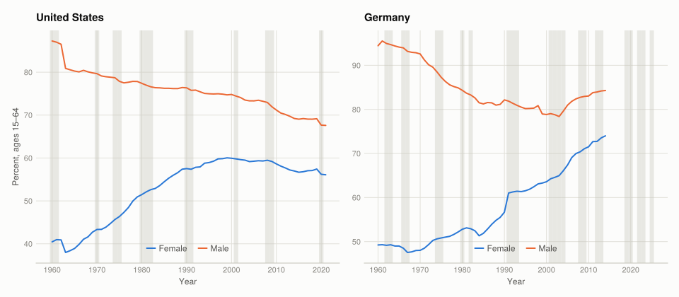
In the US, female participation climbs strongly until around 2000 while male participation falls throughout; the gap therefore narrows from both sides. German female participation also rises, but male participation begins higher and declines, leaving a persistent gap. Recessions do not explain the long trends: their shaded intervals are short, while the convergence takes decades.
The levels differ from CORE’s written US summary because the book’s workbook and its instruction are internally inconsistent: the workbook behaves like an all-adult series, while the question asks for ages 15–64. The causal story is about the trends and composition, not that denominator.
Q2. The great moderation and cyclical employment
Logs and the HP filter
Taking logs makes a deviation comparable across levels: a 1% movement has approximately the same log size in a small and a large economy. The annual HP filter chooses a smooth trend by minimizing squared departures plus λ = 6.25 times squared changes in trend growth.
for (source, stem, from) in [(:GDP, "GDP_log", 1960),
                             (:hours_worked_all, "hours_all_log", 1960),
                             (:hours_worked_female, "hours_female_log", 1960),
                             (:hours_worked_male, "hours_male_log", 1960),
                             (:labour_productivity, "productivity_log", 1960),
                             (:LFP_rate_female, "lfp_female_log", 1963),
                             (:LFP_rate_male, "lfp_male_log", 1963)]
    log_col = Symbol(stem, "_value")
    dataset_main[!, log_col] = [ismissing(x) ? missing : log(Float64(x))
                                for x in dataset_main[!, source]]
    attach_hp!(dataset_main, log_col, stem; from)
end

# CORE's derived columns are validation targets only, never analysis inputs.
core_check = hp_components(Int.(core_us_all.Year), Float64.(core_us_all[!, "Log GDP"]))
maximum(abs.(core_check.trend .- Float64.(core_us_all[!, "Log GDP (trend)"])))1.2434497875801753e-13The maximum difference from CORE’s stored US GDP trend is at floating-point noise level, which pins both the formula and endpoint convention.
fig = Figure(size = (960, 650))
for (j, country) in enumerate(COUNTRIES)
    d = dataset_main[dataset_main.Country .== country, :]
    for (i, (col, title)) in enumerate([(:GDP_log_cycle, "Log real GDP"),
                                         (:hours_all_log_cycle, "Log weekly hours")])
        ax = series_axis(fig, (i, j), dataset_main, country;
                         title = "$country — $title", ylabel = j == 1 ? "Deviation" : "")
        keep = .!ismissing.(d[!, col])
        lines!(ax, d.Year[keep], d[keep, col]; color = series_color(i))
        hlines!(ax, [0]; color = BASELINE, linewidth = 1)
    end
end
fig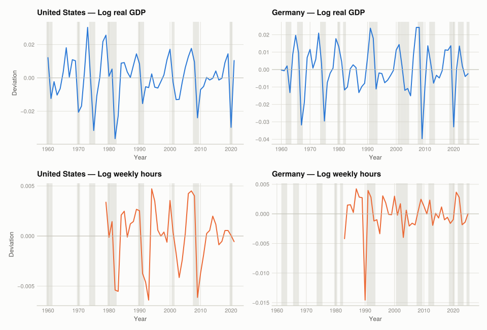
The US GDP cycle becomes visibly calmer after the severe 1980 and 1981–82 recessions: the usual start of the great moderation is the mid-1980s. The financial crisis in 2008 and the pandemic shock in 2020 are the two candidates for its end, though treating exceptional shocks as a new variance regime is a judgement rather than something this chart decides. German GDP is also less volatile after the early 1980s, with reunification and the pandemic interrupting the comparison.
Cyclicality and relative volatility
function complete_rows(df, cols)
    reduce(.&, [.!ismissing.(df[!, c]) for c in cols])
end

correlations = DataFrame(Country = String[], correlation = Float64[], years = String[])
volatility = DataFrame(Country = String[], total = Float64[], female = Float64[], male = Float64[],
                       years = String[])
for country in COUNTRIES
    d = dataset_main[dataset_main.Country .== country, :]
    pair = complete_rows(d, [:GDP_log_cycle, :hours_all_log_cycle])
    push!(correlations, (country, cor(Float64.(d[pair, :GDP_log_cycle]),
                                     Float64.(d[pair, :hours_all_log_cycle])),
                         "$(minimum(d.Year[pair]))–$(maximum(d.Year[pair]))"))

    cols = [:GDP_log_cycle, :hours_all_log_cycle,
            :hours_female_log_cycle, :hours_male_log_cycle]
    keep = complete_rows(d, cols)
    sd_gdp = std(Float64.(d[keep, :GDP_log_cycle]))
    push!(volatility, (country,
          std(Float64.(d[keep, :hours_all_log_cycle])) / sd_gdp,
          std(Float64.(d[keep, :hours_female_log_cycle])) / sd_gdp,
          std(Float64.(d[keep, :hours_male_log_cycle])) / sd_gdp,
          "$(minimum(d.Year[keep]))–$(maximum(d.Year[keep]))"))
end

correlation_table = transform(correlations, :correlation => ByRow(x -> round(x; digits = 3)) => :correlation)
volatility_table = transform(volatility,
    [:total, :female, :male] .=> ByRow(x -> round(x; digits = 3)) .=> [:total, :female, :male])
(correlation_table, volatility_table)(2×3 DataFrame Row │ Country correlation years │ String Float64 String ─────┼─────────────────────────────────────── 1 │ United States 0.724 1979–2021 2 │ Germany -0.011 1983–2025, 2×5 DataFrame Row │ Country total female male years │ String Float64 Float64 Float64 String ─────┼───────────────────────────────────────────────────── 1 │ United States 0.233 0.192 0.274 1979–2021 2 │ Germany 0.235 0.426 0.17 1983–2025)
A positive correlation means hours are procyclical: they rise above trend when GDP does. The US relationship is much stronger than Germany’s. Every relative standard deviation is below 1, so weekly hours are less volatile than GDP. In the US, male hours are more volatile than female hours, the asymmetry central to Albanesi’s explanation; Germany does not reproduce that ordering.
function period_volatility(df, country, lo, hi)
    d = df[(df.Country .== country) .& (df.Year .>= lo) .& (df.Year .<= hi), :]
    keep = complete_rows(d, [:GDP_log_cycle, :hours_female_log_cycle, :hours_male_log_cycle])
    sd_gdp = std(Float64.(d[keep, :GDP_log_cycle]))
    return (female = std(Float64.(d[keep, :hours_female_log_cycle])) / sd_gdp,
            male = std(Float64.(d[keep, :hours_male_log_cycle])) / sd_gdp)
end

split_volatility = DataFrame(Country = String[], period = String[], sex = String[], value = Float64[])
for country in COUNTRIES, (label, lo, hi) in [("1983–2007", 1983, 2007),
                                               ("2008–latest", 2008, 2025)]
    v = period_volatility(dataset_main, country, lo, hi)
    append!(split_volatility,
            DataFrame(Country = fill(country, 2), period = fill(label, 2),
                      sex = ["Female", "Male"], value = [v.female, v.male]))
end
transform(split_volatility, :value => ByRow(x -> round(x; digits = 3)) => :relative_sd)
8×5 DataFrame
| Row | Country | period | sex | value | relative_sd |
|---|---|---|---|---|---|
| String | String | String | Float64 | Float64 | |
| 1 | United States | 1983–2007 | Female | 0.230935 | 0.231 |
| 2 | United States | 1983–2007 | Male | 0.372455 | 0.372 |
| 3 | United States | 2008–latest | Female | 0.181488 | 0.181 |
| 4 | United States | 2008–latest | Male | 0.214429 | 0.214 |
| 5 | Germany | 1983–2007 | Female | 0.631201 | 0.631 |
| 6 | Germany | 1983–2007 | Male | 0.233956 | 0.234 |
| 7 | Germany | 2008–latest | Female | 0.150666 | 0.151 |
| 8 | Germany | 2008–latest | Male | 0.0988283 | 0.099 |
fig = Figure(size = (900, 400))
for (j, country) in enumerate(COUNTRIES)
    d = split_volatility[split_volatility.Country .== country, :]
    ax = Axis(fig[1, j]; title = country, ylabel = j == 1 ? "SD of hours / SD of GDP" : "",
              xticks = ([1, 2], ["1983–2007", "2008–latest"]))
    for (k, sex) in enumerate(SEXES)
        s = d[d.sex .== sex, :]
        barplot!(ax, [1, 2] .+ (k == 1 ? -0.18 : 0.18), s.value;
                 width = 0.34, color = series_color(k), label = sex)
    end
    axislegend(ax; position = :rt)
end
fig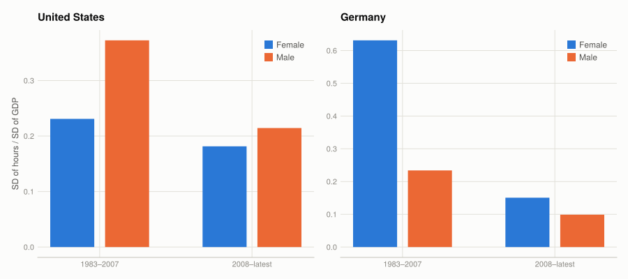
Women’s rising share in US employment put more weight on the less volatile component, damping aggregate hours. Because hours and GDP move together, that composition shift is a plausible contributor to the great moderation. It is not a complete causal test: technology, policy and sectoral change moved at the same time. Germany is a useful warning against treating “female” as intrinsically stable; its sex ordering and timing are not the same.
Q3. The productivity slowdown
The walkthrough divides one logged trend by the preceding logged trend. That is not a percentage growth rate. If t is a log trend, growth is 100 × (exp(t − lag(t)) − 1), which is what is used here.
function add_growth!(df, trend_col, out_col)
    df[!, out_col] = Vector{Union{Missing,Float64}}(missing, nrow(df))
    for country in COUNTRIES
        rows = findall((df.Country .== country) .& .!ismissing.(df[!, trend_col]))
        rows = rows[sortperm(df.Year[rows])]
        for k in 2:length(rows)
            i, prev = rows[k], rows[k-1]
            df.Year[i] == df.Year[prev] + 1 || continue
            df[i, out_col] = 100 * (exp(df[i, trend_col] - df[prev, trend_col]) - 1)
        end
    end
end
add_growth!(dataset_main, :productivity_log_trend, :productivity_growth)
add_growth!(dataset_main, :lfp_female_log_trend, :lfp_female_growth)
add_growth!(dataset_main, :lfp_male_log_trend, :lfp_male_growth)

DataFrame(Country = COUNTRIES,
          productivity_years = [let d = dataset_main[(dataset_main.Country .== c) .&
                                        .!ismissing.(dataset_main.productivity_growth), :]
                                    "$(minimum(d.Year))–$(maximum(d.Year))"
                                end for c in COUNTRIES])
2×2 DataFrame
| Row | Country | productivity_years |
|---|---|---|
| String | String | |
| 1 | United States | 1971–2021 |
| 2 | Germany | 1992–2025 |
fig = Figure(size = (960, 650))
for (j, country) in enumerate(COUNTRIES)
    d = dataset_main[dataset_main.Country .== country, :]
    ax1 = series_axis(fig, (1, j), dataset_main, country;
                      title = "$country — productivity trend", ylabel = j == 1 ? "Percent" : "")
    keep = .!ismissing.(d.productivity_growth)
    lines!(ax1, d.Year[keep], d.productivity_growth[keep]; color = series_color(1))
    hlines!(ax1, [0]; color = BASELINE, linewidth = 1)

    ax2 = series_axis(fig, (2, j), dataset_main, country;
                      title = "$country — productivity and participation",
                      ylabel = j == 1 ? "Percent" : "")
    for (k, (col, label)) in enumerate([(:productivity_growth, "Productivity"),
                                         (:lfp_female_growth, "Female LFP"),
                                         (:lfp_male_growth, "Male LFP")])
        keep = .!ismissing.(d[!, col])
        lines!(ax2, d.Year[keep], d[keep, col]; color = series_color(k), label)
    end
    axislegend(ax2; position = :rb)
end
fig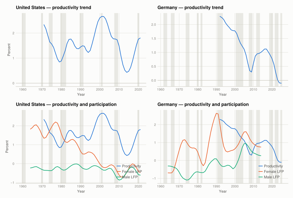
US trend productivity growth falls sharply in the 1970s, remains subdued into the 1980s, and accelerates in the 1990s. Female participation grows fastest during the first slowdown and then flattens as productivity accelerates; male participation has a persistent negative trend. One composition explanation is that new entrants initially had less measured experience, lowering average output per hour, then accumulated experience and education, raising it later.
This is timing evidence, not proof that women entering work caused the slowdown. Germany cannot supply the same 1970s test because its productivity series begins in 1991; its later data do not show the clean inverse timing needed for the same explanation.
Q4. Jobless recoveries
fig = Figure(size = (960, 760))
for (j, country) in enumerate(COUNTRIES)
    d = dataset_main[(dataset_main.Country .== country) .& (dataset_main.Year .>= 1963), :]
    for (i, (col, label)) in enumerate([(:LFP_rate_all, "All"),
                                         (:LFP_rate_female, "Female"),
                                         (:LFP_rate_male, "Male")])
        ax = series_axis(fig, (i, j), dataset_main, country;
                         title = "$country — $label", ylabel = j == 1 ? "Log LFP rate" : "")
        keep = .!ismissing.(d[!, col])
        lines!(ax, d.Year[keep], log.(Float64.(d[keep, col])); color = series_color(i))
    end
end
fig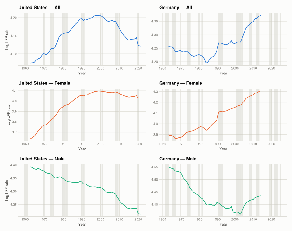
Before the 1990s, total US participation returned to or exceeded its pre-recession level quickly. After the 2001 and 2008 recessions it did not: these are jobless recoveries on the extensive margin. Male participation shows scarring after much earlier recessions too. Rising female participation had previously offset that weakness; once female participation flattened, it could no longer do so, and the aggregate series began to look like the male one.
Germany’s archived participation series shows recoveries through 2014, including the global financial crisis, but not the pandemic. Participation behaves differently enough that the US composition account is not a universal explanation.
Albanesi’s Changing Business Cycles: The Role of Women’s Employment reaches the same broad US conclusion from household microdata: growing women’s employment changes aggregate volatility, productivity dynamics and recovery patterns. The agreement matters because the data here are aggregates. The micro evidence supplies a mechanism that aggregate co-movement alone cannot.
What this project covered
| Concept | Where | In Julia |
|---|---|---|
| Read a CSV inside a ZIP | Part 1 Q1 | ZipFile.Reader, CSV.read(IOBuffer(...)) |
| Quarterly-to-annual recession dates | Part 1 Q2–Q3 | grouped maximum, adjacent-quarter checks |
| Long-to-wide reshaping | Part 1 Q4 | unstack with explicit sex labels |
| Full joins with explicit keys | Part 1 Q5 | reduce(outerjoin, ...) |
| HP trend and cycle | Part 2 Q2 | solve (I + λD′D)trend = data |
| Cyclicality | Part 2 Q2 | cor on common complete years |
| Relative volatility | Part 2 Q2 | std(hours cycle) / std(GDP cycle) |
| Growth from a log trend | Part 2 Q3 | 100 * (exp(Δtrend) - 1) |
| Recession shading | Part 2 | vspan! before the data lines |
The R → Julia page has the translation table.