9. Credit-excluded households in a developing country

Who cannot borrow, who does not bother asking, and why the second group is larger

The Ethiopian Socioeconomic Survey, 2013–14: 5,262 households, of which 1,480 borrowed. The question is who is shut out of credit — and the survey is unusually good at separating the household that asked and was refused from the household that never asked because it expected refusal.

Part 9.1 — households that did not get a loan
Part 9.2 — households that got a loan

New concepts: credit-excluded and credit-constrained households, discouraged borrowers, indicator variables built from survey answers, and selection bias. Book pages: project, R walk-through, solutions.

using XLSX, DataFrames
using Statistics
using CairoMakie
using Dates
using DoingEconomics

CairoMakie.activate!(type = "svg")
use_doingecon_theme!()

path = rawpath("09", "ethiopia-credit-ess.xlsx")
dictionary = DataFrame(XLSX.readtable(path, "Data dictionary"))
allHH = DataFrame(XLSX.readtable(path, "All households"; infer_eltypes = true))
gotL = DataFrame(XLSX.readtable(path, "Got loan"; infer_eltypes = true))

(all_households = size(allHH), got_loan = size(gotL))

(all_households = (5262, 19), got_loan = (1480, 21))

After Project 8 this file is a relief: missing values are empty cells, which XLSX.jl reads as missing directly, and nothing needs recoding from words to numbers. The dictionary covers the household characteristics:

dictionary

11×2 DataFrame

Row	Variable name	Description
	String	String
1	household_id2	Unique household ID
2	got_loan	Over the past 12 months, did anyone in this household borrow on credit from someone outside the household or from an institution for business or farming purposes, receiving either cash or inputs?
3	rural	Whether household lives in rural area, small town (urban), or large town (urban)
4	hhsize	Household size
5	region	Region
6	gender	Gender of household head
7	age	Age of household head (years)
8	young_children	Number of young children in household (13 years of age or below)
9	working_age_adults	Number of working-age adults in household (aged between 14 to 54)
10	max_education	Highest education level attained by anyone in the household (number of years of schooling)
11	number_assets	Number of assets owned by household (the sum of all items in Section 10 of the questionnaire)

Eleven variables described, but allHH has nineteen columns. The credit variables are the ones not documented — loan_rejected, rejection_source1 and 2, did_not_apply, reason_not_apply1 and 2, loan_purpose and loan_purpose_other. Section 14 of the ESS household questionnaire has the question wording, and Part 9.1 is largely about turning those answers into indicators.

did_not_apply is named for one answer and coded for the other

DataFrame(variable = ["did_not_apply", "loan_rejected", "rural"],
          values = [join(sort(unique(skipmissing(allHH[!, c]))), " | ")
                    for c in ["did_not_apply", "loan_rejected", "rural"]])

3×2 DataFrame

Row	variable	values
	String	String
1	did_not_apply	Applied \| Did not apply
2	loan_rejected	No \| Yes
3	rural	Large town (urban) \| Rural \| Small town (urban)

did_not_apply takes the values "Applied" and "Did not apply", so the name reads as a negation while the values read as a statement. Writing did_not_apply == "Applied" looks like a mistake and is correct; writing did_not_apply == true would be a mistake and looks fine. Every filter below spells out the string.

Part 9.1 — Households that did not get a loan

Q1. Where these households are, and who they are

(a) Region by area type. Each row is a region and the first three columns are that region’s split between large towns, small towns and rural areas, so they sum across to 1. The last column is the region’s share of the whole sample.

const AREAS = ["Rural", "Small town (urban)", "Large town (urban)"]

region_table = DataFrame(region = String[], rural = Float64[], small_town = Float64[],
                         large_town = Float64[], share_of_sample = Float64[])
for r in sort(unique(skipmissing(allHH.region)))
    rows = allHH[coalesce.(allHH.region .== r, false), :]
    push!(region_table, (r, [round(count(==(a), skipmissing(rows.rural)) / nrow(rows),
                                   digits = 2) for a in AREAS]...,
                         round(nrow(rows) / nrow(allHH), digits = 2)))
end
show_all(region_table)

11×5 DataFrame

Row	region	rural	small_town	large_town	share_of_sample
	String	Float64	Float64	Float64	Float64
1	Addis Ababa	0.0	0.0	1.0	0.06
2	Afar	0.76	0.15	0.1	0.03
3	Amhara	0.67	0.11	0.22	0.2
4	Benshagul Gumuz	0.9	0.1	0.0	0.02
5	Diredwa	0.53	0.0	0.47	0.04
6	Gambelia	0.8	0.08	0.12	0.02
7	Harari	0.73	0.0	0.27	0.03
8	Oromia	0.61	0.11	0.28	0.2
9	SNNP	0.73	0.09	0.18	0.23
10	Somalie	0.76	0.09	0.16	0.06
11	Tigray	0.56	0.07	0.37	0.12

Table 1: Area type within each region, and each region’s share of the sample. Reproduces the book’s Solution figure 9.1.

All eleven regions reproduce the published table. 63% of the sample is rural, and the regional variation is the thing to notice: Addis Ababa is 100% large-town by construction, while Benshagul Gumuz is 90% rural. Three regions — Amhara, Oromia and SNNP — hold 63% of all households between them.

(b) Female household heads.

female = count(==("Female"), skipmissing(allHH.gender))
(female_heads = female,
 gender_recorded = count(!ismissing, allHH.gender),
 pct_of_all = round(100 * female / nrow(allHH), digits = 2),
 pct_of_recorded = round(100 * female / count(!ismissing, allHH.gender), digits = 2))

(female_heads = 1599, gender_recorded = 5261, pct_of_all = 30.39, pct_of_recorded = 30.39)

30.39%, against the book’s 30.40%. One household has no gender recorded, and neither denominator gives 30.40 — the last digit is a rounding difference in the published figure, not a different sample.

(c) The household characteristics.

allHH.female = [g === missing ? missing : Float64(g == "Female") for g in allHH.gender]

const CHARS = ["hhsize" => "Household size", "female" => "Gender (1 = female head)",
               "age" => "Age of household head", "young_children" => "Young children",
               "working_age_adults" => "Working-age adults",
               "max_education" => "Max education (years)",
               "number_assets" => "Number of assets"]

summary_table = DataFrame(variable = String[], mean = Float64[], sd = Float64[],
                          min = Float64[], max = Float64[], n = Int[])
for (col, label) in CHARS
    x = Float64.(collect(skipmissing(allHH[!, col])))
    push!(summary_table, (label, round(mean(x), digits = 2), round(std(x), digits = 2),
                          minimum(x), maximum(x), length(x)))
end
summary_table

7×6 DataFrame

Row	variable	mean	sd	min	max	n
	String	Float64	Float64	Float64	Float64	Int64
1	Household size	4.58	2.4	1.0	16.0	5260
2	Gender (1 = female head)	0.3	0.46	0.0	1.0	5261
3	Age of household head	44.18	15.61	3.0	99.0	5253
4	Young children	1.89	1.71	0.0	10.0	5262
5	Working-age adults	2.58	1.52	0.0	10.0	5262
6	Max education (years)	7.53	7.28	0.0	30.0	5262
7	Number of assets	14.9	17.23	0.0	203.0	5262

Table 2: Household demographics, all 5,262 households. Reproduces the book’s Solution figure 9.2.

Every mean and standard deviation matches the published table.

(d) What the tables say. The typical household is 4.58 people — call it five — with one or two young children and two or three working-age adults. Its head is 44 and its most educated member has 7.5 years of schooling, which is primary plus a little. It owns about 15 assets.

The spreads matter more than the averages, because they are what the credit analysis will be about:

Assets: mean 14.9, SD 17.2, max 203. The standard deviation exceeds the mean, so the distribution is strongly right-skewed and the mean is not the typical household. This is the variable most likely to serve as collateral, and it is the least evenly held.
Education: mean 7.5, SD 7.3, min 0. Again SD ≈ mean. A substantial share of households have nobody with any schooling, while the maximum is 30 years.
Age min 3. A three-year-old household head is not a household head. It is either a coding error or a household recorded by a child’s age after some other loss; either way it is a reminder that survey extremes deserve a look before they enter a regression.

Q2. Applications and rejections

(a) The cross-tabulation, with missing values kept as their own row and column, because the point of the table is to find the responses that should not exist.

label(v) = v === missing ? "Blank" : string(v)
const APPLY = ["Applied", "Did not apply", "Blank"]
const REJECT = ["No", "Yes", "Blank"]

crosstab = DataFrame(application = String[], not_rejected = Int[], rejected = Int[],
                     blank = Int[], total = Int[])
for a in APPLY
    counts = [count(i -> label(allHH.did_not_apply[i]) == a &&
                         label(allHH.loan_rejected[i]) == b, 1:nrow(allHH)) for b in REJECT]
    push!(crosstab, (a, counts..., sum(counts)))
end
push!(crosstab, ("Total", [sum(crosstab[!, c]) for c in
                           [:not_rejected, :rejected, :blank]]..., nrow(allHH)))
crosstab

4×5 DataFrame

Row	application	not_rejected	rejected	blank	total
	String	Int64	Int64	Int64	Int64
1	Applied	1363	201	1	1565
2	Did not apply	3632	24	2	3658
3	Blank	37	2	0	39
4	Total	5032	227	3	5262

Table 3: Loan applications against rejections, all responses including blanks. Reproduces the book’s Solution figure 9.3.

(b) Which responses cannot be true. Two cells are contradictory, because both questions cover the same twelve months:

24 households say they did not apply and were also rejected. A loan cannot be refused if it was never requested.
2 households give no answer on applying but report a rejection.

Dropping those, plus the 39 blank-application and 3 blank-rejection rows, leaves the three cells the book keeps:

sane = allHH[.!ismissing.(allHH.did_not_apply) .& .!ismissing.(allHH.loan_rejected) .&
             .!((allHH.did_not_apply .== "Did not apply") .&
                (allHH.loan_rejected .== "Yes")), :]

sane.HH_status = [r.did_not_apply == "Applied" ?
                  (r.loan_rejected == "No" ? "successful" : "denied") : "did not apply"
                  for r in eachrow(sane)]

applicants = sane[sane.did_not_apply .== "Applied", :]
(usable = nrow(sane),
 dropped = nrow(allHH) - nrow(sane),
 applied = nrow(applicants),
 pct_applied = round(100 * nrow(applicants) / nrow(sane), digits = 2),
 pct_successful_of_applicants =
     round(100 * count(==("successful"), applicants.HH_status) / nrow(applicants), digits = 2))

(usable = 5196, dropped = 66, applied = 1564, pct_applied = 30.1, pct_successful_of_applicants = 87.15)

5,196 households remain and 30.10% of them applied — both match the book.

The published success rate uses the wrong denominator

The question asks: of the households that applied, what percentage were successful? The Solutions page answers 96.13%. The data says 87.15%.

Where 96.13 comes from:

rejected = count(==("denied"), sane.HH_status)
successful = count(==("successful"), sane.HH_status)

DataFrame(quantity = ["successful ÷ applicants  (the question asked)",
                      "100 − rejected ÷ all usable  (the published 96.13)",
                      "rejected ÷ applicants",
                      "rejected ÷ all usable"],
          value = round.([100 * successful / nrow(applicants),
                          100 - 100 * rejected / nrow(sane),
                          100 * rejected / nrow(applicants),
                          100 * rejected / nrow(sane)], digits = 2))

4×2 DataFrame

Row	quantity	value
	String	Float64
1	successful ÷ applicants (the question asked)	87.15
2	100 − rejected ÷ all usable (the published 96.13)	96.13
3	rejected ÷ applicants	12.85
4	rejected ÷ all usable	3.87

96.13% is the rejected households as a share of all 5,196, subtracted from 100. It divides by the whole sample where the question divides by applicants.

This is not a rounding difference. 12.85% of applicants were turned down, not 3.87% — a rejection rate more than three times what the published figure implies, and the difference between “credit is almost freely available to those who ask” and “one applicant in eight is refused.”

The book’s very next sentence uses 3.87% correctly, as a share of all households. The two denominators are crossed inside a single paragraph, which is what makes it easy to miss: both numbers are individually right about something, and neither answers the question above it.

(c) Which category is which. The three surviving cells map onto the concepts unevenly, and the mapping is the substance of this Part.

DataFrame(category = ["Applied, got a loan", "Applied, refused", "Did not apply"],
          n = [successful, rejected, count(==("did not apply"), sane.HH_status)],
          pct = round.(100 .* [successful, rejected,
                               count(==("did not apply"), sane.HH_status)] ./ nrow(sane),
                       digits = 2))

3×3 DataFrame

Row	category	n	pct
	String	Int64	Float64
1	Applied, got a loan	1363	26.23
2	Applied, refused	201	3.87
3	Did not apply	3632	69.9

Table 4: The three usable response patterns as shares of the 5,196 households.

Applied and refused (3.87%) is credit excluded. These households wanted to borrow at the going terms and could not, which is the definition.
Applied and got a loan (26.23%) is not credit excluded, but may still be credit constrained. Receiving a loan says nothing about the terms. A household that borrowed at 200% interest from a moneylender got credit and was still constrained by it — and Part 9.2 shows such loans exist in this data.
Did not apply (69.90%) is unclassifiable from this table alone, and it is by far the largest group. It contains households with no need to borrow, households that expected refusal, and households deterred by the terms. Separating them needs the reasons, which is Q3.

That ordering is the point of the Part. The group the two questions can classify cleanly is the smallest one, and the group that matters most for measuring exclusion is the one the questions cannot classify at all.

Q3. Discouraged borrowers and credit-constrained households

Two indicators built from the two free-response reason fields.

reasons(r) = [x for x in (r.reason_not_apply1, r.reason_not_apply2) if x !== missing]

# Discouraged: expected refusal, so never asked.
sane.discouraged = [Int("Believe Would Be Refused" in reasons(r)) for r in eachrow(sane)]

# Constrained: gave any reason other than no-need or unclassifiable.
const NOT_CONSTRAINED = ["Other (Specify)", "Have Adequate Farm"]
sane.credit_constrained = [Int(any(!in(x, NOT_CONSTRAINED) for x in reasons(r)))
                           for r in eachrow(sane)]

DataFrame(indicator = ["Discouraged borrowers", "Credit constrained"],
          n = [sum(sane.discouraged), sum(sane.credit_constrained)],
          pct = round.(100 .* [mean(sane.discouraged), mean(sane.credit_constrained)],
                       digits = 2))

2×3 DataFrame

Row	indicator	n	pct
	String	Int64	Float64
1	Discouraged borrowers	588	11.32
2	Credit constrained	3012	57.97

588 discouraged (11.32%) and 3,012 credit constrained (57.97%), both matching the book.

Put those beside Q2: the credit-excluded group the survey can identify directly is 3.87% of households, while the credit-constrained group is 57.97% — fifteen times larger. Measuring exclusion by rejections alone would miss almost all of it.

Both definitions are choices, and the book says so about the first. Two things worth being explicit about:

“Discouraged” here means only "Believe Would Be Refused". A household answering "Inadequate Collateral" or "Too Expensive" is arguably also discouraged — it has assessed the terms and concluded there is no point. The narrow definition makes 11.32% a lower bound.
“Constrained” is broad by comparison, excluding only "Have Adequate Farm" (no need) and "Other (Specify)" (unclassifiable). It therefore counts "Do Not Like To Be In Debt" as a constraint, which is a preference rather than a constraint. That makes 57.97% an upper bound, and the largest single reason falls in exactly this contested category.

The two indicators bracket the truth rather than measuring it, and Q4’s reason tables show why the bracket is wide.

Q4. Why households did not apply

function reason_shares(col)
    vals = collect(skipmissing(sane[!, col]))
    Dict(r => count(==(r), vals) / length(vals) for r in unique(vals)), length(vals)
end

first_shares, n_first = reason_shares("reason_not_apply1")
second_shares, n_second = reason_shares("reason_not_apply2")

reason_table = DataFrame(reason = collect(keys(first_shares)),
                         most_important = round.(collect(values(first_shares)), digits = 2))
reason_table.second_most = [round(get(second_shares, r, 0.0), digits = 2)
                            for r in reason_table.reason]
sort!(reason_table, :most_important, rev = true)
(n_giving_a_first_reason = n_first, n_giving_a_second_reason = n_second)

(n_giving_a_first_reason = 3566, n_giving_a_second_reason = 1995)

Table 5: Reasons for not applying for a loan, as proportions of the households giving each answer. Reproduces the book’s Solution figures 9.4 and 9.5.

reason_table

10×3 DataFrame

Row	reason	most_important	second_most
	String	Float64	Float64
1	Do Not Like To Be In Debt	0.19	0.24
2	Have Adequate Farm	0.19	0.05
3	Fear Not Be Able To Pay	0.17	0.28
4	Believe Would Be Refused	0.12	0.09
5	No Farm or Business	0.1	0.04
6	Do Not Know Any Lender	0.07	0.06
7	Inadequate Collateral	0.05	0.09
8	Too Expensive	0.05	0.07
9	Other (Specify)	0.04	0.02
10	Too Much Trouble	0.03	0.06

Both columns reproduce the published tables. Note the denominators: 3,566 households gave a first reason but only 1,995 gave a second, so the two columns are shares of different groups and are not directly comparable as a pair.

fig = Figure(size = (900, 520))
ax = Axis(fig[1, 1];
          title = "Debt aversion and fear of non-payment dominate both rankings",
          xlabel = "Share of households giving a reason at that rank",
          yticks = (1:nrow(reason_table), reverse(reason_table.reason)),
          limits = ((0, 0.32), nothing))

positions = collect(nrow(reason_table):-1:1)
for (j, (col, lab)) in enumerate([(:most_important, "Most important reason"),
                                  (:second_most, "Second most important")])
    barplot!(ax, positions .+ (j == 1 ? 0.19 : -0.19), reason_table[!, col];
             direction = :x, width = 0.34, color = series_color(j), label = lab)
end
Legend(fig[0, 1], ax; orientation = :horizontal, framevisible = false)
fig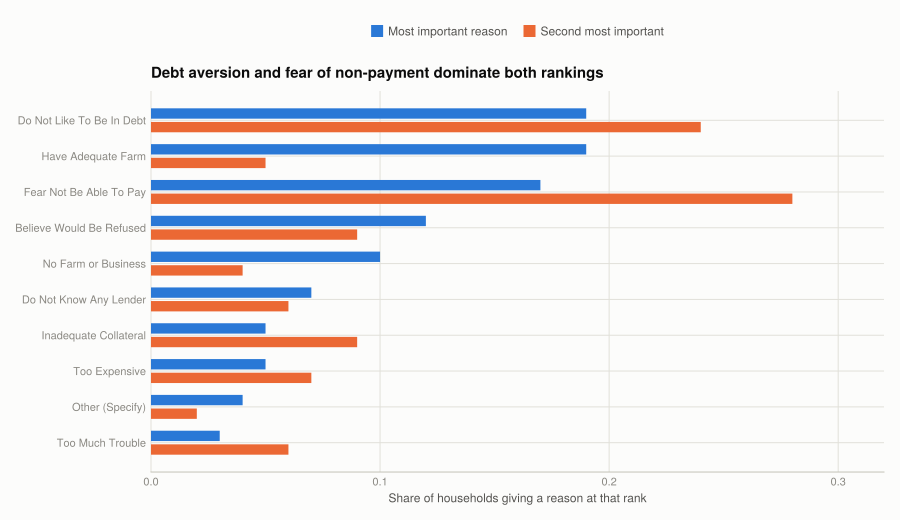

Figure 1: Reasons for not applying for a loan. Two series, so the reason’s rank carries the colour; shares are of the households giving a reason at that rank, which is why the columns do not sum across. Bars are dodged with a surface gap rather than stacked, because these are shares of two different denominators and a stack would imply a total.

The most common answers are not about supply. "Do Not Like To Be In Debt" is the joint largest first reason at 0.19 and the second largest second reason at 0.24. "Have Adequate Farm" ties it at 0.19 among first reasons — a household saying it does not need a loan.

Between them, those two answers account for roughly 38% of first reasons, and they mean opposite things for this project: one is a preference, the other is an absence of demand. Neither is a credit market failing to serve a household that wants credit.

The reasons that do indicate a constraint are, taken together, comparable in size. "Fear Not Be Able To Pay" (0.17 first, 0.28 second — the largest second reason), "Believe Would Be Refused" (0.12), "Too Expensive" (0.05), "Inadequate Collateral" (0.05) and "Do Not Know Any Lender" (0.07) describe households that assessed their prospects and stopped.

"Do Not Know Any Lender" at 0.07 is worth singling out. It is not a price or a collateral problem; it is an information problem, and it implies a different remedy from the others.

This is the evidence that Q3’s 57.97% is an upper bound. Most of the gap between 11.32% and 57.97% is "Do Not Like To Be In Debt" and "Fear Not Be Able To Pay" — the first a preference, the second ambiguous between a constraint and a realistic assessment of one’s own income risk.

Q5. Successful against denied borrowers

Loan purpose first. The book flags a data problem here: in allHH the purpose recorded for every successful household is "Other", so the successful column has to come from the gotL sheet instead.

denied_rows = sane[sane.HH_status .== "denied", :]

function purpose_shares(vals)
    v = collect(skipmissing(vals))
    Dict(string(p) => count(==(p), v) / length(v) for p in unique(v)), length(v)
end
succ_shares, n_succ = purpose_shares(gotL.loan_purpose)
den_shares, n_den = purpose_shares(denied_rows.loan_purpose)

# `union` of two key sets is a Set, which has no ordering — collect before sorting.
purpose_table = DataFrame(purpose = sort(collect(union(keys(succ_shares),
                                                       keys(den_shares)))))
purpose_table.successful = [round(get(succ_shares, p, 0.0), digits = 3)
                            for p in purpose_table.purpose]
purpose_table.denied = [round(get(den_shares, p, 0.0), digits = 3)
                        for p in purpose_table.purpose]
sort!(purpose_table, :successful, rev = true)
(successful_n = n_succ, denied_n = n_den, columns_sum =
     round.([sum(purpose_table.successful), sum(purpose_table.denied)], digits = 3))

(successful_n = 1444, denied_n = 195, columns_sum = [1.001, 1.0])

Table 6: Loan purpose for successful and denied applicants, as proportions. Successful purposes come from the “Got loan” sheet; denied from “All households”. Reproduces the book’s Solution figure 9.6.

purpose_table

9×3 DataFrame

Row	purpose	successful	denied
	String	Float64	Float64
1	Purchase Agricultural Inputs for Food Crop	0.3	0.21
2	For consumption and personal expenses	0.202	0.0
3	Business Start-up Capital	0.155	0.262
4	Purchase Non-farm Inputs	0.114	0.026
5	Purchase Inputs for other Crops	0.098	0.062
6	Expanding Business	0.082	0.138
7	Other (Specify)	0.027	0.256
8	Purchase House/Lease Land	0.023	0.031
9	10	0.0	0.015

Solution figure 9.6’s successful column sums to 0.91

The published table lists 0.01 for "Purchase Inputs for other Crops" among successful borrowers. The data gives 0.098. Their own column is the check: with 0.01 it sums to 0.91, and with 0.10 it sums to 1.00. It is a dropped decimal place, not a different sample — every other cell in both columns reproduces.

The comparison is not clean, and the book says why. "For consumption and personal expenses" is its own category for successful borrowers (0.202) but is folded into "Other (Specify)" for denied ones — which is most of why denied borrowers show 0.256 on "Other" against 0.027 for successful. The free-text field confirms the size:

(households_with_other_text = count(!ismissing, allHH.loan_purpose_other),)

(households_with_other_text = 52,)

52 households wrote in a reason, so the consumption share among denied applicants cannot be reconstructed at anything like 20%. The two columns should not be differenced on "Other" or on consumption.

What survives the incomparability:

Business start-up is the largest denied purpose (0.262) and less than half that among successful (0.155). Together with "Expanding Business" (0.138 against 0.082), business lending is where refusal concentrates. Start-up capital has no track record and often no collateral, which is what a lender prices.
Agricultural inputs for food crops is the largest successful purpose (0.300) against 0.210 denied. Short, seasonal, and against a harvest a lender can anticipate.
"10" appears as a purpose for 0.015 of denied households. It is not a category in the survey — a code that escaped its labels.

Household characteristics.

const COMPARE = ["age" => "Age of household head",
                 "max_education" => "Highest education in household",
                 "number_assets" => "Number of assets", "hhsize" => "Household size",
                 "young_children" => "Number of young children",
                 "working_age_adults" => "Number of working-age adults"]

chars_table = DataFrame(characteristic = String[], successful = Float64[], denied = Float64[])
for (col, lab) in COMPARE
    push!(chars_table, (lab,
        [round(mean(skipmissing(sane[sane.HH_status .== st, col])), digits = 2)
         for st in ["successful", "denied"]]...))
end
pushfirst!(chars_table, ("Number of observations", Float64(successful), Float64(rejected)))
chars_table

7×3 DataFrame

Row	characteristic	successful	denied
	String	Float64	Float64
1	Number of observations	1363.0	201.0
2	Age of household head	43.37	41.21
3	Highest education in household	7.26	8.0
4	Number of assets	15.88	14.46
5	Household size	4.87	4.82
6	Number of young children	2.09	2.22
7	Number of working-age adults	2.75	2.76

Table 7: Mean household characteristics for successful and denied applicants. Reproduces the book’s Solution figure 9.7.

How each characteristic should matter, before looking. A lender is pricing the probability of repayment:

Age — an older head has had longer to accumulate assets and a repayment record. Expect successful borrowers to be older.
Education — more schooling means higher and steadier income. Expect successful to be more educated.
Assets — the collateral channel, and the most direct of the six. Expect successful to own more.
Household size — more members to service the debt, but also more claims on income. Sign ambiguous.
Young children — dependants who consume now and earn later. Ambiguous, and negative in the short run.
Working-age adults — earning capacity. Expect successful to have more.

Three of the six go the expected way, and the largest surprise is education. Successful borrowers are 2.2 years older (43.37 against 41.21) and own 1.4 more assets (15.88 against 14.46). But their households are less educated — 7.26 years against 8.00.

That is backwards on the repayment story, and the likely reason is that education drives application rather than approval. A more educated household knows lenders exist, knows how to apply, and is confident enough to try — so it appears in the applicant pool more often, including in its rejected tail. The comparison here conditions on having applied, so it cannot separate “education makes approval more likely” from “education makes applying more likely.” Q6 shows this difference is not measured precisely enough to lean on either way.

Household size, children and working-age adults are all essentially identical between the two groups.

Q6. Are those differences real?

Six differences in means with 95% confidence intervals, using the standard error for a difference between independent groups from Project 8.

const Z = 1.96

differences = DataFrame(characteristic = String[], successful = Float64[], sd_s = Float64[],
                        n_s = Int[], denied = Float64[], sd_d = Float64[], n_d = Int[],
                        difference = Float64[], lower = Float64[], upper = Float64[],
                        excludes_zero = Bool[])
for (col, lab) in COMPARE
    x = Float64.(collect(skipmissing(sane[sane.HH_status .== "successful", col])))
    y = Float64.(collect(skipmissing(sane[sane.HH_status .== "denied", col])))
    d = mean(x) - mean(y)
    se = sqrt(var(x) / length(x) + var(y) / length(y))
    push!(differences, (lab, round(mean(x), digits = 2), round(std(x), digits = 2), length(x),
                        round(mean(y), digits = 2), round(std(y), digits = 2), length(y),
                        round(d, digits = 3), round(d - Z * se, digits = 2),
                        round(d + Z * se, digits = 2), abs(d) > Z * se))
end
differences

6×11 DataFrame

Row	characteristic	successful	sd_s	n_s	denied	sd_d	n_d	difference	lower	upper	excludes_zero
	String	Float64	Float64	Int64	Float64	Float64	Int64	Float64	Float64	Float64	Bool
1	Age of household head	43.37	14.27	1361	41.21	12.85	201	2.154	0.22	4.09	true
2	Highest education in household	7.26	6.74	1363	8.0	7.9	201	-0.735	-1.88	0.41	false
3	Number of assets	15.88	19.0	1363	14.46	16.84	201	1.421	-1.12	3.96	false
4	Household size	4.87	2.35	1362	4.82	2.35	201	0.047	-0.3	0.39	false
5	Number of young children	2.09	1.68	1363	2.22	1.8	201	-0.135	-0.4	0.13	false
6	Number of working-age adults	2.75	1.49	1363	2.76	1.42	201	-0.003	-0.21	0.21	false

Table 8: Differences in mean characteristics, successful minus denied, with 95% confidence intervals. Reproduces the book’s Solution figure 9.9.

All six reproduce the published intervals.

Here the book’s interval arithmetic is correct

Project 8’s Solutions page computed confidence intervals with a combined standard deviation over the pooled sample size, which understated every width. Solution figure 9.9 uses the right formula and this page matches it to the second decimal. The error there was local to that page, not a convention running through the book.

sorted_diff = sort(differences, :difference)

fig = Figure(size = (880, 500))
ax = Axis(fig[1, 1];
          title = "Only age differs measurably between successful and denied applicants",
          ylabel = "Difference in means (successful − denied)",
          xticks = (1:nrow(sorted_diff), sorted_diff.characteristic),
          xticklabelrotation = pi / 7,
          limits = (nothing, (-2.5, 5.0)))
hlines!(ax, [0]; color = BASELINE, linewidth = 1)
barplot!(ax, 1:nrow(sorted_diff), sorted_diff.difference;
         width = 0.5, color = series_color(1))
errorbars!(ax, 1:nrow(sorted_diff), sorted_diff.difference,
           sorted_diff.difference .- sorted_diff.lower,
           sorted_diff.upper .- sorted_diff.difference;
           color = INK_SECONDARY, whiskerwidth = 12, linewidth = 2)
fig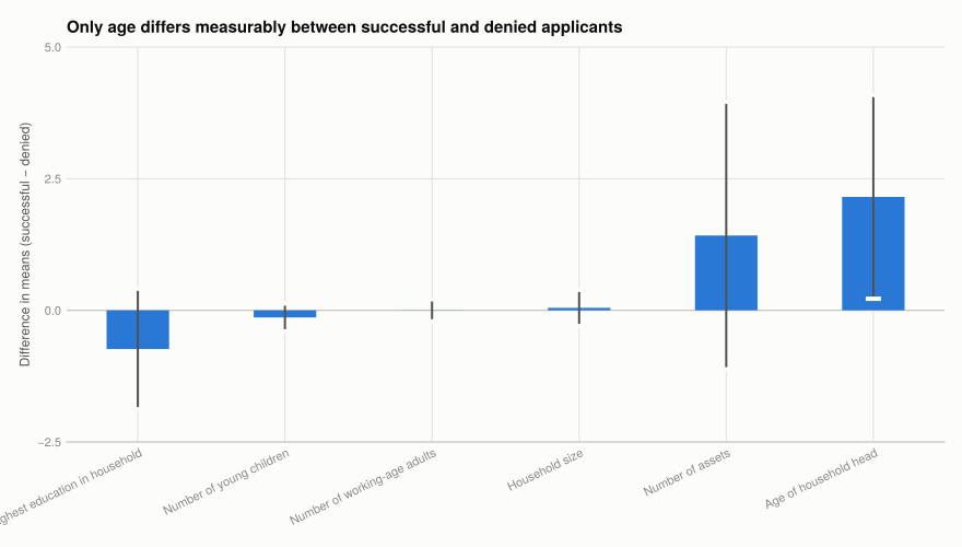

Figure 2: Difference in mean characteristics, successful minus denied applicants, sorted. One series, so one colour; error bars are the 95% half-widths from the table above and the rule at zero is what each is read against. Age and assets are plotted on the same axis as counts of people because all six are differences in whatever unit the characteristic uses — the axis is a difference, not a level.

One of the six differences excludes zero. Age: 2.15 years [0.22, 4.09], and only just — the lower bound is a fifth of a year from zero. Assets, the difference with the clearest mechanism, is 1.42 [−1.12, 3.96]: the interval is nearly three times the estimate.

The reason is visible in the table. There are 201 denied households against 1,361 successful ones, and the standard error of a difference is dominated by the smaller group. On assets, the denied group’s SD of 16.8 over 201 observations contributes about six times the variance that 1,361 successful households contribute.

So the honest reading is that this comparison cannot distinguish successful from denied applicants on five of six characteristics, and the education result that looked like a puzzle in Q5 has an interval of [−1.88, 0.41] — comfortably including zero. It is not a finding that needs explaining; it is noise, and the explanation offered in Q5 is a hypothesis rather than a result.

What would help. More denied households, which the survey cannot supply — refusal is rare, so a nationally representative sample of 5,262 yields only 201. That is a structural feature of studying exclusion from a general household survey, and it is why the next question widens the comparison to groups the survey has more of.

Q7. Four groups, not two

Successful and denied applicants, plus the discouraged and the credit constrained. The last two overlap with each other and with “did not apply”, which is why they are shown as separate columns rather than a partition.

const GROUPS = ["successful" => sane.HH_status .== "successful",
                "denied" => sane.HH_status .== "denied",
                "discouraged" => sane.discouraged .== 1,
                "constrained" => sane.credit_constrained .== 1]

four_groups = DataFrame(characteristic = ["Number of observations";
                                          [lab for (_, lab) in COMPARE]])
for (label, mask) in GROUPS
    rows = sane[mask, :]
    four_groups[!, label] = [Float64(nrow(rows));
                             [round(mean(skipmissing(rows[!, col])), digits = 2)
                              for (col, _) in COMPARE]]
end
four_groups

7×5 DataFrame

Row	characteristic	successful	denied	discouraged	constrained
	String	Float64	Float64	Float64	Float64
1	Number of observations	1363.0	201.0	588.0	3012.0
2	Age of household head	43.37	41.21	43.28	44.84
3	Highest education in household	7.26	8.0	6.5	7.14
4	Number of assets	15.88	14.46	10.16	13.54
5	Household size	4.87	4.82	4.65	4.44
6	Number of young children	2.09	2.22	2.03	1.81
7	Number of working-age adults	2.75	2.76	2.49	2.49

Table 9: Mean characteristics across four borrower types. Discouraged and credit-constrained overlap, so the columns are not mutually exclusive. Reproduces the book’s Solution figure 9.11.

Every value matches the published table.

fig = Figure(size = (960, 560))
labels = [lab for (_, lab) in COMPARE]
names_ = [label for (label, _) in GROUPS]

for (k, lab) in enumerate(labels)
    row, col = fldmod1(k, 3)
    values = Float64[four_groups[four_groups.characteristic .== lab, g][1] for g in names_]
    ax = Axis(fig[row, col];
              title = lab, titlesize = 12,
              xticks = (1:4, names_), xticklabelrotation = pi / 6,
              limits = (nothing, (0, maximum(values) * 1.25)))
    barplot!(ax, 1:4, values; width = 0.55, color = series_color(1))
    for (x, v) in zip(1:4, values)
        text!(ax, x, v; text = string(v), fontsize = 9,
              align = (:center, :bottom), offset = (0, 3))
    end
end
fig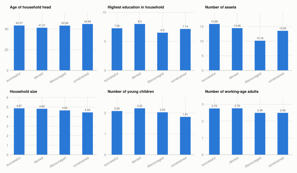

Figure 3: Each characteristic across the four borrower types, one panel per characteristic so that variables on different scales keep their own axis. One series throughout — the group is a category on the horizontal axis, not a colour, which keeps the four bars comparable within each panel.

Discouraged households are the asset-poor ones. They own 10.16 assets against 15.88 for successful borrowers and 14.46 for denied ones — a gap of about a third, and far larger than any difference Q6 could measure. They also have the least education of the four groups, at 6.50 years.

This is the useful result of the Part, and it comes from the group the survey classifies least directly. The households that never applied because they expected refusal look materially poorer than the households that applied and were refused. If exclusion were measured by rejections alone, the most disadvantaged group would be invisible.

Credit-constrained households are the smallest ones: household size 4.44 against 4.87, young children 1.81 against 2.09, working-age adults 2.49. Their head is also the oldest at 44.84. But this group is 3,012 households — 58% of the sample — so its means are close to the sample averages almost by construction, and the comparison is less informative than the discouraged column.

Selection bias, and why it matters here. Every comparison in Part 9.1 conditions on an outcome the household influenced. Q5 and Q6 compare applicants only, so they measure the effect of characteristics on approval among households that chose to apply — and the choice to apply depends on the same characteristics. If more educated households are more likely to apply including when their prospects are marginal, then the applicant pool’s education gap tells you about applying, not about approval, which is exactly the ambiguity Q5 hit.

The general form: estimating a relationship on a sample selected by the outcome recovers the selection as much as the relationship. A study of what makes countries prosper that uses only countries publishing good statistics is drawing from a sample whose membership depends on state capacity — itself a determinant of prosperity. The estimate absorbs the selection.

What would fix it here is data on the terms households expected, so that the decision not to apply could be modelled rather than conditioned away. The survey records reasons but not expected prices, so the four groups can be described and compared, and that is as far as this design goes.

Part 9.2 — Households that got a loan

1,480 loans, with start and end dates, amount, interest, and source. The dates need cleaning first, and one of the problems is not a problem.

Q1. Loan duration

(a) What is wrong with the date fields.

date_values = DataFrame(field = String[], value = String[], n = Int[])
for c in ["loan_startyear", "loan_endyear"]
    vals = collect(skipmissing(gotL[!, c]))
    for v in sort(unique(vals); by = string)
        push!(date_values, (c, string(v), count(==(v), vals)))
    end
end
show_all(date_values)

18×3 DataFrame

Row	field	value	n
	String	String	Int64
1	loan_startyear	1996	1
2	loan_startyear	1999	1
3	loan_startyear	200	1
4	loan_startyear	2002	2
5	loan_startyear	2003	1
6	loan_startyear	2004	12
7	loan_startyear	2005	758
8	loan_startyear	2006	700
9	loan_startyear	3	1
10	loan_endyear	1	1
11	loan_endyear	2003	1
12	loan_endyear	2005	8
13	loan_endyear	2006	696
14	loan_endyear	2007	186
15	loan_endyear	2008	32
16	loan_endyear	2009	16
17	loan_endyear	2010	5
18	loan_endyear	2012	1

Table 10: Every distinct value in the four date fields, with counts. The year fields are where the errors are.

DataFrame(field = ["loan_startmonth", "loan_endmonth"],
          distinct = [join(sort(unique(string.(skipmissing(gotL[!, c])))), ", ")
                      for c in ["loan_startmonth", "loan_endmonth"]])

2×2 DataFrame

Row	field	distinct
	String	String
1	loan_startmonth	April, August, December, February, January, July, June, March, May, November, October, September
2	loan_endmonth	April, August, December, February, January, July, June, March, May, November, October, Pagume, September

Three impossible years — "3" and "200" as start years, "1" as an end year — each appearing once. "200" is plainly a truncated "2005" or "2006", but there is no way to tell which, so guessing would invent data; all three become missing.

“Pagume” is a real month

loan_endmonth contains Pagume, which looks like a data error and is not. The Ethiopian calendar has thirteen months: twelve of 30 days, then Pagume, a five- or six-day intercalary month falling in early September on the Gregorian calendar.

So it maps to September rather than to missing. This is the kind of thing that is only visible if you look at the distinct values before cleaning — an automated “drop what isn’t a month name” rule would silently discard valid observations, and a survey of Ethiopian households is exactly where a thirteenth month should be expected.

(b) and (c) Dates, and how much is missing.

const MONTHS = Dict("January" => 1, "February" => 2, "March" => 3, "April" => 4,
                    "May" => 5, "June" => 6, "July" => 7, "August" => 8,
                    "September" => 9, "October" => 10, "November" => 11,
                    "December" => 12,
                    # Pagume is the 13th Ethiopian month, in early September.
                    "Pagume" => 9)

parse_year(y) = y === missing ? missing :
                (n = tryparse(Int, string(y));
                 n === nothing || n < 1990 || n > 2015 ? missing : n)
parse_month(m) = m === missing ? missing : get(MONTHS, string(m), missing)

gotL.start_year = parse_year.(gotL.loan_startyear)
gotL.start_month = parse_month.(gotL.loan_startmonth)
gotL.end_year = parse_year.(gotL.loan_endyear)
gotL.end_month = parse_month.(gotL.loan_endmonth)

as_date(y, m) = (y === missing || m === missing) ? missing : Date(y, m)
gotL.start_date = as_date.(gotL.start_year, gotL.start_month)
gotL.end_date = as_date.(gotL.end_year, gotL.end_month)

DataFrame(date = ["Start date", "End date"],
          missing_n = [count(ismissing, gotL.start_date), count(ismissing, gotL.end_date)],
          missing_pct = [round(100 * count(ismissing, gotL.start_date) / nrow(gotL), digits = 2),
                         round(100 * count(ismissing, gotL.end_date) / nrow(gotL), digits = 2)])

2×3 DataFrame

Row	date	missing_n	missing_pct
	String	Int64	Float64
1	Start date	6	0.41
2	End date	535	36.15

6 start dates missing (0.41%) and 535 end dates (36.15%), both matching the book.

The asymmetry is the finding, not the total. Start dates are essentially complete; more than a third of end dates are absent. That is not random non-response — a loan with no end date is most naturally a loan that had not ended when the survey was taken. If so, the missing third is disproportionately long loans, and every duration statistic below is computed on a sample biased toward loans short enough to have finished. It is the same selection problem as Q7, arriving through missingness instead of through a filter.

(d) and (e) Duration, and the negative ones.

gotL.duration = [(s === missing || e === missing) ? missing : Dates.value(e - s)
                 for (s, e) in zip(gotL.start_date, gotL.end_date)]

# Two treatments of a negative duration: drop it, or assume the dates were swapped.
gotL.duration_dropped = [x === missing ? missing : (x < 0 ? missing : x)
                         for x in gotL.duration]
gotL.loan_length = [x === missing ? missing : abs(x) for x in gotL.duration]

computable = collect(skipmissing(gotL.duration))
(computable = length(computable),
 negative = count(<(0), computable),
 negative_pct = round(100 * count(<(0), computable) / length(computable), digits = 1),
 range_days = extrema(computable))

(computable = 943, negative = 172, negative_pct = 18.2, range_days = (-1066, 4748))

943 loans have both dates, and 172 of them — 18.2% — end before they begin. That is far too many to be a handful of typos, and it makes the choice of treatment consequential rather than cosmetic:

Dropping them leaves 771 loans and assumes the affected records are uninformative.
Taking the absolute value keeps all 943 and assumes the two dates were transposed, so the magnitude is right and only the order is wrong.

The book uses the absolute value for what follows, so this page does too — but with 18% of computable durations affected, the two treatments are different samples, not the same sample cleaned two ways. Note also that the most extreme negative is −1,066 days, nearly three years, which is hard to read as a transcription slip and easier to read as a genuinely confused pair of dates.

(f) Long-term loans.

gotL.long_term = [x === missing ? missing : Int(x > 365) for x in gotL.loan_length]
classified = collect(skipmissing(gotL.long_term))

(with_a_duration = length(classified),
 long_term = sum(classified),
 short_term = count(iszero, classified),
 unclassified = count(ismissing, gotL.long_term),
 pct_long_term = round(100 * mean(classified), digits = 2))

(with_a_duration = 943, long_term = 215, short_term = 728, unclassified = 537, pct_long_term = 22.8)

22.80% of classifiable loans ran longer than a year — 215 of 943, matching the book, with 537 loans unclassifiable.

The denominator deserves the emphasis the headline number usually gets. 537 of 1,480 loans — 36% — have no duration at all, and by the argument above they are the ones most likely to be long. So 22.80% is a lower bound on the long-term share, and possibly a substantial underestimate.

Q2. Amounts and interest rates

(a) The distribution of loan size.

amount = Float64.(collect(skipmissing(gotL.loan_amount)))
paired = [(Float64(r.loan_amount), Float64(r.loan_interest)) for r in eachrow(gotL)
          if r.loan_amount !== missing && r.loan_interest !== missing]
total = [a + i for (a, i) in paired]

DataFrame(measure = ["Loan amount (principal)", "Total amount to repay"],
          n = [length(amount), length(total)],
          mean = round.([mean(amount), mean(total)]),
          sd = round.([std(amount), std(total)]),
          min = [minimum(amount), minimum(total)],
          max = [maximum(amount), maximum(total)])

2×6 DataFrame

Row	measure	n	mean	sd	min	max
	String	Int64	Float64	Float64	Float64	Float64
1	Loan amount (principal)	1479	26896.0	783587.0	1.0	3.0e7
2	Total amount to repay	1445	29223.0	827144.0	20.0	3.126e7

Table 11: Loan principal and total repayable, in Ethiopian birr. Reproduces the book’s Solution figure 9.12.

Both rows match the published table. The mean is meaningless here and the reason is in the same row. A mean of 26,896 birr with a standard deviation of 783,587 — twenty-nine times the mean — and a range from 1 birr to 30 million. One loan is 1,100 times the mean.

A single observation is doing most of the work, which is why the quartiles in (d) are the honest summary and the mean is not.

(b) and (c) Interest rates, and the extreme observation.

gotL.rate = [(r.loan_amount === missing || r.loan_interest === missing ||
              r.loan_amount == 0) ? missing :
             100 * r.loan_interest / r.loan_amount for r in eachrow(gotL)]
rates = collect(skipmissing(gotL.rate))

(with_a_rate = length(rates),
 zero_interest_pct = round(100 * count(iszero, rates) / length(rates), digits = 2),
 median = round(median(rates), digits = 2),
 max = round(maximum(rates), digits = 0))

(with_a_rate = 1445, zero_interest_pct = 50.52, median = 0.0, max = 20000.0)

50.52% of loans carry no interest at all, matching the book, and the maximum rate is 20,000%.

The book calls this loan “200%”

The Solutions page describes the extreme observation as having an interest rate of 200%. The interest is 200 times the principal, so as a percentage that is 20,000% — their rate is the ratio, not multiplied by 100.

The observation identified is the same one either way, and it is excluded from what follows on both readings. Only the units differ, and this page states rates as percentages throughout.

plotted = [(a, r) for (a, r) in zip(gotL.loan_amount, gotL.rate)
           if a !== missing && r !== missing && a > 0 && r > 0]
extreme = argmax(last.(plotted))

fig = Figure(size = (880, 500))
ax = Axis(fig[1, 1];
          title = "One loan sits two orders of magnitude above every other rate",
          xlabel = "Loan principal (birr, log scale)",
          ylabel = "Interest rate (%, log scale)",
          xscale = log10, yscale = log10)
scatter!(ax, first.(plotted), last.(plotted); color = series_color(1), markersize = 7)
text!(ax, first(plotted[extreme]), last(plotted[extreme]);
      text = "excluded: $(round(Int, last(plotted[extreme])))%", fontsize = 11,
      align = (:left, :center), offset = (10, 0), color = INK)
text!(ax, 1.5, 1.2;
      text = "$(count(iszero, rates)) zero-interest loans are not shown\n" *
             "(a log axis has no zero)",
      fontsize = 10, align = (:left, :bottom), color = MUTED)
fig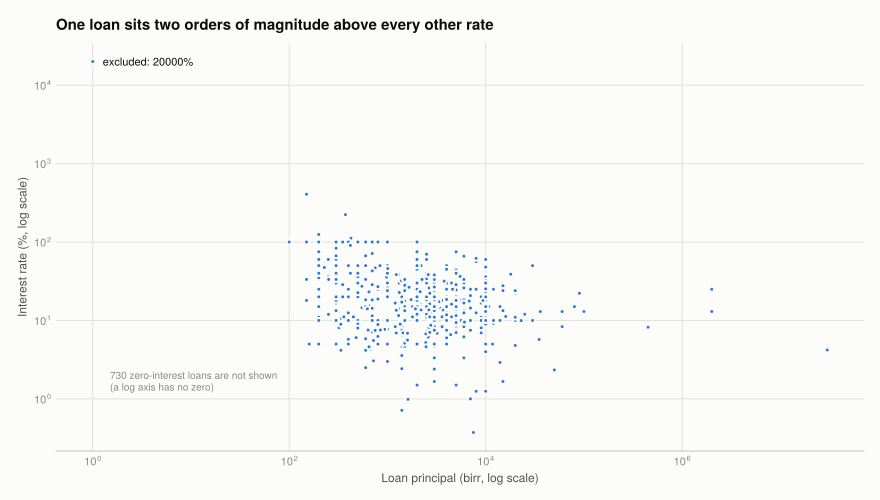

Figure 4: Interest rate against loan principal, both on log scales because each spans four to five orders of magnitude. One series, so one colour; the single excluded observation is labelled rather than given a colour of its own. Zero-interest loans cannot be drawn on a log axis and are counted in the annotation instead.

(d) By term. Excluding the one extreme observation.

keep = [r !== missing && r < 10_000 for r in gotL.rate]

by_term = DataFrame(measure = String[], term = String[], n = Int[], mean = Float64[],
                    sd = Float64[], min = Float64[], q1 = Float64[], median = Float64[],
                    q3 = Float64[], max = Float64[])
for (measure, col, digits) in [("Loan amount", :loan_amount, 0), ("Interest rate (%)", :rate, 2)]
    for (term, flag) in ["Long term" => 1, "Short term" => 0]
        mask = keep .& coalesce.(gotL.long_term .== flag, false)
        v = Float64.(collect(skipmissing(gotL[mask, col])))
        push!(by_term, (measure, term, length(v), round(mean(v); digits),
                        round(std(v); digits), round(minimum(v); digits),
                        round(quantile(v, 0.25); digits), round(median(v); digits),
                        round(quantile(v, 0.75); digits), round(maximum(v); digits)))
    end
end
by_term

4×10 DataFrame

Row	measure	term	n	mean	sd	min	q1	median	q3	max
	String	String	Int64	Float64	Float64	Float64	Float64	Float64	Float64	Float64
1	Loan amount	Long term	211	172718.0	2.07274e6	20.0	1000.0	3700.0	8000.0	3.0e7
2	Loan amount	Short term	717	3017.0	8398.0	40.0	480.0	1500.0	3500.0	150000.0
3	Interest rate (%)	Long term	211	18.9	26.79	0.0	0.0	14.08	24.52	223.53
4	Interest rate (%)	Short term	717	11.01	17.25	0.0	0.0	5.0	17.14	111.76

Table 12: Loan amount and interest rate by term, excluding the single extreme-rate observation. Reproduces the book’s Solution figure 9.14.

Every cell matches the published table.

Long-term loans are larger, and far more unequally sized. Median 3,700 birr against 1,500 for short-term — a factor of 2.5 at the median. But the means are 172,718 against 3,017, a factor of 57, because the 30-million-birr loan is long term. Comparing medians and comparing means gives answers an order of magnitude apart, and the median is the one to trust.

Long-term loans also charge more. Median rate 14.08% against 5.00%, and mean 18.90% against 11.01%. Both terms have a first quartile of 0.00%, so at least a quarter of loans in each group are interest-free.

That last fact is the interesting one, and it does not fit a market story. A quarter of loans at zero interest in both terms suggests two different lending arrangements coexisting rather than a single market pricing risk — which is what Q3 tests by looking at who the lender was.

(e) Interest rates against household characteristics.

rate_corr = DataFrame(characteristic = String[], correlation = Float64[], n = Int[])
for (col, lab) in COMPARE
    ok = keep .& .!ismissing.(gotL[!, col])
    push!(rate_corr, (lab, round(cor(Float64.(gotL[ok, col]), Float64.(gotL[ok, :rate])),
                                 digits = 3), count(ok)))
end
sort!(rate_corr, :correlation)
rate_corr

6×3 DataFrame

Row	characteristic	correlation	n
	String	Float64	Int64
1	Highest education in household	-0.084	1444
2	Number of assets	-0.047	1444
3	Age of household head	0.026	1443
4	Number of working-age adults	0.047	1444
5	Number of young children	0.102	1444
6	Household size	0.105	1442

Table 13: Correlation between the interest rate charged and household characteristics, excluding the extreme observation.

Reading the interest rate as a price for default risk, the expectation is that households with more assets and more earners pay less, and households with more dependants pay more.

fig = Figure(size = (860, 460))
ax = Axis(fig[1, 1];
          title = "No household characteristic explains much of the rate charged",
          ylabel = "Correlation with interest rate",
          xticks = (1:nrow(rate_corr), rate_corr.characteristic),
          xticklabelrotation = pi / 7,
          limits = (nothing, (-0.5, 0.5)))
hlines!(ax, [0]; color = BASELINE, linewidth = 1)
barplot!(ax, 1:nrow(rate_corr), rate_corr.correlation;
         width = 0.5, color = series_color(1))
for (x, v) in zip(1:nrow(rate_corr), rate_corr.correlation)
    text!(ax, x, v; text = string(v), fontsize = 10,
          align = (:center, v < 0 ? :top : :bottom), offset = (0, v < 0 ? -4 : 4))
end
fig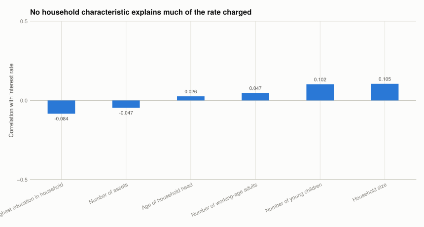

Figure 5: Correlation between interest rate charged and each household characteristic. One series; the zero rule is the reference. All six correlations are small — the axis is deliberately not stretched to fill the panel, because doing so would make weak associations look strong.

Every correlation is small. Nothing about the household explains much of what it was charged, which is itself the answer: if these rates were priced on household default risk, the characteristics a lender can observe should show up here, and they barely do.

The alternative explanation is that the rate is set by which lender the household reached rather than by the household’s own risk — a moneylender and a relative charge differently for the same borrower. That is Q3.

Q3. Who lends

sources = sort(unique(skipmissing(gotL.borrowed_from)))
source_table = DataFrame(source = String[])
for a in AREAS
    source_table[!, a] = Int[]
end
source_table.total = Int[]
for s in sources
    rows = gotL[coalesce.(gotL.borrowed_from .== s, false), :]
    counts = [count(==(a), skipmissing(rows.rural)) for a in AREAS]
    push!(source_table, (s, counts..., nrow(rows)))
end
sort!(source_table, :total, rev = true)
show_all(source_table)

10×5 DataFrame

Row	source	Rural	Small town (urban)	Large town (urban)	total
	String	Int64	Int64	Int64	Int64
1	Relative	329	42	168	539
2	Microfinance Institution	286	26	63	375
3	Neighbour	118	7	38	163
4	Other (specify)	123	4	19	146
5	Grocery/Local Merchant	50	10	26	86
6	NGO	49	5	4	58
7	Money Lender (Katapila)	49	2	1	52
8	Religious Institution	21	0	1	22
9	Employer	2	1	16	19
10	Bank (commercial)	4	0	6	10

Table 14: Source of finance by area type, counts. Reproduces the structure of the book’s Solution figure for R walk-through 9.11.

Relatives are the single largest source of credit — 539 loans, more than a third of the total — followed by microfinance institutions at 375. Commercial banks made 10 loans out of 1,480.

Grouping by what kind of institution each is:

const LENDER_TYPE = Dict(
    "Bank (commercial)" => "Formal", "Employer" => "Formal",
    "Microfinance Institution" => "Microfinance", "NGO" => "Microfinance",
    "Relative" => "Informal", "Neighbour" => "Informal",
    "Money Lender (Katapila)" => "Informal", "Grocery/Local Merchant" => "Informal",
    "Religious Institution" => "Informal", "Other (specify)" => "Other")

gotL.lender_type = [s === missing ? missing : LENDER_TYPE[string(s)] for s in gotL.borrowed_from]
types = collect(skipmissing(gotL.lender_type))

type_table = DataFrame(lender_type = unique(types))
type_table.loans = [count(==(t), types) for t in type_table.lender_type]
type_table.pct = round.(100 .* type_table.loans ./ length(types), digits = 1)
type_table.median_rate = [round(median(skipmissing(gotL[coalesce.(gotL.lender_type .== t,
                                                                 false) .& keep, :rate])),
                                digits = 2) for t in type_table.lender_type]
type_table.zero_interest_pct =
    [round(100 * mean(iszero,
                      collect(skipmissing(gotL[coalesce.(gotL.lender_type .== t, false) .&
                                               keep, :rate]))), digits = 1)
     for t in type_table.lender_type]
sort!(type_table, :loans, rev = true)
type_table

4×5 DataFrame

Row	lender_type	loans	pct	median_rate	zero_interest_pct
	String	Int64	Float64	Float64	Float64
1	Informal	862	58.6	0.0	79.8
2	Microfinance	433	29.5	15.0	5.4
3	Other	146	9.9	10.7	17.2
4	Formal	29	2.0	6.0	42.3

Table 15: Sources grouped by type of lender. Formal excludes microfinance, which is treated separately because it is neither an informal relationship nor a commercial bank.

This is where the zero-interest loans come from. Informal lenders — relatives, neighbours, local merchants, religious institutions and moneylenders — make 58.6% of all loans, and 79.8% of them charge nothing. Their median rate is 0.00%. Microfinance institutions and NGOs make 29.5% of loans at a median of 15.00%, with only 5.4% interest-free.

That resolves the puzzle from Q2. Half of all loans carry no interest not because Ethiopian credit is cheap, but because half of it is not priced credit at all: informal zero-interest lending alone accounts for about 47% of every loan in the file, which is most of the 50.52% zero-interest share. A loan from a relative at 0% and a microfinance loan at 15% are different instruments, and averaging them produces a “market interest rate” that describes neither.

The formal category — commercial banks and employers — is 29 loans out of 1,480, so its median of 6.00% rests on too little data to compare. That scarcity is itself the finding: formal finance is close to absent for these households.

It also explains why household characteristics barely correlate with the rate. The rate is mostly determined by which of these two systems the household borrowed in, and that is a question about the household’s network and location rather than its balance sheet — which is why the rural/urban split in the source table is the more informative cut.

area_shares = DataFrame(source = source_table.source)
for a in AREAS
    n_area = count(==(a), skipmissing(gotL.rural))
    area_shares[!, a] = round.(source_table[!, a] ./ n_area, digits = 3)
end
show_all(area_shares)

10×4 DataFrame

Row	source	Rural	Small town (urban)	Large town (urban)
	String	Float64	Float64	Float64
1	Relative	0.317	0.429	0.49
2	Microfinance Institution	0.275	0.265	0.184
3	Neighbour	0.114	0.071	0.111
4	Other (specify)	0.118	0.041	0.055
5	Grocery/Local Merchant	0.048	0.102	0.076
6	NGO	0.047	0.051	0.012
7	Money Lender (Katapila)	0.047	0.02	0.003
8	Religious Institution	0.02	0.0	0.003
9	Employer	0.002	0.01	0.047
10	Bank (commercial)	0.004	0.0	0.017

Table 16: Each source’s loans as a share of that area type’s loans, so columns sum to 1 and areas of very different size can be compared.

Microfinance is a rural institution in this data and moneylenders are almost entirely rural, while employer loans and commercial banks are concentrated in large towns. Relatives lend everywhere.

(d) What is missing from the data. Three things that the questions above kept running into:

The terms that were offered but refused. Every rate here is a rate somebody accepted. The households in Part 9.1 that did not apply because credit was "Too Expensive" faced a price that this dataset does not record, so the distribution of offered rates cannot be recovered from the distribution of accepted ones — the same selection problem as Q7, now on the price rather than the quantity.
Loan duration for the third of loans still outstanding. No end date means no duration, and those are the loans most likely to be long.
Whether the loan was repaid, which loan_repaid records but which cannot be interpreted without knowing whether the term had ended. Default is the outcome the interest rate is supposed to be pricing, and it is the one thing this data cannot check the pricing against.

Collateral offered, the household’s prior borrowing history, and distance to the nearest lender would each address a specific gap above. The last is the one that would speak most directly to "Do Not Know Any Lender" — 7% of first reasons in Q4.

What this project covered

Concept	Where	In Julia
Reading several sheets separately	Setup	`XLSX.readtable(path, "Got loan")`
Cross-tabulation keeping blanks	Q9.1 Q2	`count` over a labelling function
Indicators from free-response fields	Q9.1 Q3	`Int(any(...))` over the reason columns
Row-proportion tables	Q9.1 Q1	divide each row by its own total
Difference in means with a CI	Q9.1 Q6	`sqrt(var(x)/nx + var(y)/ny)`, `± 1.96se`
Asymmetric error bars	Q9.1 Q6	`errorbars!(ax, x, y, low, high)`
Small multiples over a variable list	Q9.1 Q7	`fldmod1(k, 3)` for the grid position
Guarded string-to-number parsing	Q9.2 Q1	`tryparse` plus a plausible-range check
Dates from separate month and year	Q9.2 Q1	`Date(year, month)`, `Dates.value(a - b)`
A non-Gregorian month name	Q9.2 Q1	map `"Pagume"` to September, not to `missing`
Log scales on both axes	Q9.2 Q2	`xscale = log10, yscale = log10`
Quartiles beside a skewed mean	Q9.2 Q2	`quantile(v, [0.25, 0.5, 0.75])`
Every row of a long table	Q9.1 Q1	`show_all(df)`

The R → Julia page has the full translation table.