using XLSX, DataFrames
using Statistics, StatsBase, HypothesisTests
using CairoMakie
using DoingEconomics

CairoMakie.activate!(type = "svg")
use_doingecon_theme!()8. Measuring the non-monetary cost of unemployment
What 129,515 survey respondents say about life satisfaction, and how much of the work is cleaning
The European Values Study, four waves between 1981 and 2010, 164,997 respondents across 46 countries. The question is whether unemployed people report lower life satisfaction than employed people, and whether that gap is larger where the social norm of working is stronger.
- Part 8.1 — cleaning and summarizing the data
- Part 8.2 — visualizing the data
- Part 8.3 — confidence intervals for a difference in means
New concept: the confidence interval for a difference in means. But most of this project is data cleaning — the file arrives with missing values coded as the string .a, ordinal scales stored as words, one column packing two variables, and four waves that do not ask the same questions. Book pages: project, R walk-through, solutions.
Part 8.1 — Cleaning and summarizing the data
Q1. Import the four waves and label the variables
(a) The workbook holds one sheet per wave. All four share the same 17 columns, so they stack directly — reduce(vcat, ...) is the Julia equivalent of the book’s repeated rbind.
const WAVES = ["1981-1984", "1990-1993", "1999-2001", "2008-2010"]
path = rawpath("08", "life-satisfaction-evs.xlsx")

evs = reduce(vcat, [DataFrame(XLSX.readtable(path, "Wave $i")) for i in 1:4])

DataFrame(wave = WAVES, number = 1:4,
          respondents = [sum(evs.S002EVS .== w) for w in WAVES])
4×3 DataFrame
| Row | wave | number | respondents |
|---|---|---|---|
| String | Int64 | Int64 | |
| 1 | 1981-1984 | 1 | 19378 |
| 2 | 1990-1993 | 2 | 38213 |
| 3 | 1999-2001 | 3 | 41125 |
| 4 | 2008-2010 | 4 | 66281 |
164,997 rows and 17 columns. The variable names are EVS codes, which carry no meaning on their own.
(b) The workbook’s Data dictionary sheet is an empty template — it lists the 17 codes with blank name and description columns for you to fill in from the codebook PDF. Two of its rows are worth noting: it lists S009 (a country ISO code), which is not actually in the data, and it omits nothing else.
R attaches labels with attr, which stores a positional vector alongside the frame. Julia’s DataFrames has per-column metadata instead, keyed by column name:
labels = [
    "S002EVS" => ("EVS wave", "Survey wave"),
    "S003"    => ("Country", "Country or region"),
    "S006"    => ("Respondent", "Original respondent number"),
    "A009"    => ("Health", "State of health (subjective)"),
    "A170"    => ("Life satisfaction", "Satisfaction with your life as a whole"),
    "C036"    => ("Work Q1", "To develop talents you need to have a job"),
    "C037"    => ("Work Q2", "Humiliating to receive money without working for it"),
    "C038"    => ("Work Q3", "People who don't work become lazy"),
    "C039"    => ("Work Q4", "Work is a duty towards society"),
    "C041"    => ("Work Q5", "Work comes first even if it means less spare time"),
    "X001"    => ("Sex", "Sex"),
    "X003"    => ("Age", "Age in years"),
    "X007"    => ("Marital status", "Marital status"),
    "X011_01" => ("Children", "How many living children do you have"),
    "X025A"   => ("Education", "Educational level (ISCED one digit)"),
    "X028"    => ("Employment", "Employment status"),
    "X047D"   => ("Income", "Monthly household income (thousands of PPP euros)"),
]

for (col, (label, description)) in labels
    colmetadata!(evs, col, "label", label; style = :note)
    colmetadata!(evs, col, "description", description; style = :note)
end

DataFrame(variable = first.(labels),
          label = [l for (_, (l, _)) in labels],
          description = [d for (_, (_, d)) in labels])
17×3 DataFrame
| Row | variable | label | description |
|---|---|---|---|
| String | String | String | |
| 1 | S002EVS | EVS wave | Survey wave |
| 2 | S003 | Country | Country or region |
| 3 | S006 | Respondent | Original respondent number |
| 4 | A009 | Health | State of health (subjective) |
| 5 | A170 | Life satisfaction | Satisfaction with your life as a whole |
| 6 | C036 | Work Q1 | To develop talents you need to have a job |
| 7 | C037 | Work Q2 | Humiliating to receive money without working for it |
| 8 | C038 | Work Q3 | People who don't work become lazy |
| 9 | C039 | Work Q4 | Work is a duty towards society |
| 10 | C041 | Work Q5 | Work comes first even if it means less spare time |
| 11 | X001 | Sex | Sex |
| 12 | X003 | Age | Age in years |
| 13 | X007 | Marital status | Marital status |
| 14 | X011_01 | Children | How many living children do you have |
| 15 | X025A | Education | Educational level (ISCED one digit) |
| 16 | X028 | Employment | Employment status |
| 17 | X047D | Income | Monthly household income (thousands of PPP euros) |
Note
colmetadata! beats attr for exactly one reason
R’s attr(df, "labels") is a vector matched to columns by position. Drop a column or reorder one and every label after it silently points at the wrong variable — and the book’s own code then indexes it with attr(df, "labels")[attr(df, "names") == "X028"], which is the workaround for that fragility.
Julia’s metadata is keyed by column, and style = :note makes it survive the operations that would break a positional vector:
wave4_only = select(evs[evs.S002EVS .== last(WAVES), :], :X028, :A170)

(columns = names(wave4_only),
 still_labelled = colmetadata(wave4_only, :X028, "description"))
(columns = ["X028", "A170"], still_labelled = "Employment status")A filter and a select that reversed the column order, and the label is still attached to the right variable.
Q2. Whether these self-reports can be compared at all
(a) Life satisfaction (A170) across people and countries. The 1–10 answers are numbers, but treating them as a measured quantity needs three assumptions, and they get progressively harder to accept.
- Ordinality within a person — that a respondent’s 7 is more satisfied than their 6. This is the weak assumption and it is fine.
- Cardinality — that the step from 6 to 7 is the same size as the step from 8 to 9. Every mean in this project needs this. There is no reason it holds, and reported scales tend to compress at the top: moving 9 → 10 is a bigger real change than 5 → 6.
- Interpersonal and cross-country comparability — that your 7 and my 7 describe the same internal state. This is the one that actually bites for this project, because the whole design compares country averages. Translation of the question, norms about admitting dissatisfaction, and the tendency to answer near the scale midpoint all vary systematically by country.
The third assumption is where the project’s conclusions are most exposed. It matters less than it looks, though, because the analysis in Parts 8.2 and 8.3 works with differences between groups inside the same country. Any country-level offset — a national habit of answering high, a translation that shifts the whole scale — cancels out of a within-country difference. What does not cancel is a country-level difference in how unemployed people specifically respond, which is precisely the social-norm channel under study. The design cannot separate “the unemployed are less satisfied” from “the unemployed report their satisfaction differently.”
(b) Misreporting employment status (X028). Self-reported status is a single choice among eight categories, so misreporting is likely and, worse, likely non-random. Three mechanisms:
- Stigma. If unemployment is shameful — the premise of the whole project — some unemployed respondents will report “housewife”, “student”, or “self employed” instead. This is correlated with the outcome and with the country’s work ethic, so it biases the estimate in the direction of the hypothesis being tested.
- Ambiguity. Someone with a few hours of casual work, or unemployed but retraining, has a genuine choice of answers. The category set is not a partition of real situations.
- Reference period. No date is attached. Someone laid off last week may still answer “full time”.
The stigma channel is the damaging one because it is the same variable as the explanatory mechanism. Note the direction: it removes the most-ashamed unemployed people from the unemployed category, which biases the measured gap downward in high-stigma countries — against the paper’s hypothesis, not for it.
(c) Response biases in the work-attitude items (C036–C041). Three that apply here:
- Acquiescence bias — a tendency to agree with whatever is asserted. All five work items are phrased in the pro-work direction (“work is a duty towards society”), so acquiescence inflates the work-ethic score with no reverse-coded item to offset it. Check: the average would sit above the 3.0 midpoint everywhere, and the five items would correlate positively with each other more strongly than their content warrants. The observed means are 3.72 for men and 3.64 for women, both well above the 3.0 midpoint, which is consistent with this.
- Social desirability — reporting the answer that reflects well on you. Its signature is country-level: it would make the work-ethic measure track the local norm about what one ought to say rather than individual belief, which is a problem because the country average is exactly what Part 8.2 uses. Check: compare against a behavioural measure such as actual hours worked; a norm-driven score should predict stated attitudes better than behaviour.
- Anchoring to the scale midpoint — using the middle option as a default. Check: look for an excess mass at exactly 3.0 in the five-item average. Because the average of five whole numbers lands on multiples of 0.2, a genuine spike at 3.0 is visible in the frequency tables in Part 8.2 Q1.
Q3. Recoding
Five separate problems. Taking them in order.
(a) Missing values arrive as the string .a. This is the conversion artefact that does the most damage, because a single .a in a column forces every value in it to be stored as text — so nothing is numeric until it is fixed.
DataFrame(variable = names(evs),
          dot_a = [count(v -> v isa AbstractString && strip(v) == ".a", evs[!, c])
                   for c in names(evs)],
          stored_as = [string(eltype(evs[!, c])) for c in names(evs)])
17×3 DataFrame
| Row | variable | dot_a | stored_as |
|---|---|---|---|
| String | Int64 | String | |
| 1 | S002EVS | 0 | String |
| 2 | S003 | 0 | String |
| 3 | S006 | 0 | Int64 |
| 4 | A009 | 42093 | String |
| 5 | A170 | 1400 | Any |
| 6 | C036 | 61170 | String |
| 7 | C037 | 61637 | String |
| 8 | C038 | 61115 | String |
| 9 | C039 | 61586 | String |
| 10 | C041 | 61153 | String |
| 11 | X001 | 98 | String |
| 12 | X003 | 604 | Any |
| 13 | X007 | 962 | String |
| 14 | X011_01 | 99324 | Any |
| 15 | X025A | 99331 | String |
| 16 | X028 | 1645 | String |
| 17 | X047D | 83536 | Any |
for col in names(evs)
    evs[!, col] = [(v isa AbstractString && strip(v) == ".a") ? missing : v
                   for v in evs[!, col]]
end
sum(count(ismissing, evs[!, c]) for c in names(evs))635654(b) Life satisfaction mixes numbers with words. The endpoints of the scale were exported as their labels, so A170 contains 2–9 as text plus "Dissatisfied" and "Satisfied".
num(x) = x === missing ? missing :
         x isa Number ? Float64(x) : tryparse(Float64, string(x))

evs.A170 = [v === missing ? missing :
            v == "Dissatisfied" ? 1.0 :
            v == "Satisfied"    ? 10.0 : num(v) for v in evs.A170]

extrema(skipmissing(evs.A170))
(1.0, 10.0)(c) Number of children has "No children" where it means zero.
evs.X011_01 = [v === missing ? missing : v == "No children" ? 0.0 : num(v)
               for v in evs.X011_01]
extrema(skipmissing(evs.X011_01))
(0.0, 16.0)(d) Two ordinal scales stored as words. The five work items and subjective health both need numbers before they can be averaged.
const AGREE = Dict("Strongly disagree" => 1.0, "Disagree" => 2.0,
                   "Neither agree nor disagree" => 3.0,
                   "Agree" => 4.0, "Strongly agree" => 5.0)
const HEALTH = Dict("Very poor" => 1.0, "Poor" => 2.0, "Fair" => 3.0,
                    "Good" => 4.0, "Very good" => 5.0)
const WORK_ITEMS = ["C036", "C037", "C038", "C039", "C041"]

for col in WORK_ITEMS
    evs[!, col] = [v === missing ? missing : AGREE[v] for v in evs[!, col]]
end
evs.A009 = [v === missing ? missing : HEALTH[v] for v in evs.A009]
evs.X003 = num.(evs.X003)
evs.X047D = num.(evs.X047D)

DataFrame(item = vcat(WORK_ITEMS, "A009"),
          answered = [count(!ismissing, evs[!, c]) for c in vcat(WORK_ITEMS, "A009")],
          mean = [round(mean(skipmissing(evs[!, c])), digits = 3)
                  for c in vcat(WORK_ITEMS, "A009")])
6×3 DataFrame
| Row | item | answered | mean |
|---|---|---|---|
| String | Int64 | Float64 | |
| 1 | C036 | 103827 | 3.905 |
| 2 | C037 | 103360 | 3.493 |
| 3 | C038 | 103882 | 3.7 |
| 4 | C039 | 103411 | 3.67 |
| 5 | C041 | 103844 | 3.309 |
| 6 | A009 | 122904 | 3.737 |
Indexing AGREE[v] directly rather than get(AGREE, v, num(v)) is deliberate: if the file ever contains a label not in the map, this throws instead of silently producing a missing.
(e) Education packs a code and a description into one cell. X025A looks like "3 : (Upper) secondary education" — the ISCED level and its name, separated by a colon. Splitting on " : " gives a numeric level and a text description.
parts = [v === missing ? missing : split(string(v), " : ") for v in evs.X025A]
evs.Education_1 = [p === missing ? missing : num(first(p)) for p in parts]
evs.Education_2 = [p === missing ? missing :
                   (length(p) > 1 ? String(strip(p[2])) : missing) for p in parts]

levels = [(code, desc) for (code, desc) in zip(evs.Education_1, evs.Education_2)
          if code !== missing]
sort!(unique!(levels); by = first)
DataFrame(isced = first.(levels), description = last.(levels))
7×2 DataFrame
| Row | isced | description |
|---|---|---|
| Float64 | String | |
| 1 | 0.0 | Pre-primary education or none education |
| 2 | 1.0 | Primary education or first stage of basic education |
| 3 | 2.0 | Lower secondary or second stage of basic education |
| 4 | 3.0 | (Upper) secondary education |
| 5 | 4.0 | Post-secondary non-tertiary education |
| 6 | 5.0 | First stage of tertiary education |
| 7 | 6.0 | Second stage of tertiary education |
Q4. Dropping incomplete observations, wave by wave
This is the step where it is easy to destroy the dataset. The four waves do not ask the same questions, so a single dropmissing across all variables would delete every respondent in waves that never asked one of them — silently, and with no error.
The book’s filter therefore has four tiers. A170, X003, X028, X007 and X001 are required in all waves; subjective health only in waves 1, 2 and 4; the work items and income only in waves 3 and 4; children and education only in wave 4.
complete_in(df, cols) = [all(!ismissing(row[c]) for c in cols) for row in eachrow(df)]

# Keep a row unless its wave asked these questions and it left one blank.
function require_complete(df, cols; asked_in)
    keep = .!in.(df.S002EVS, Ref(asked_in)) .| complete_in(df, cols)
    return df[keep, :]
end

steps = DataFrame(step = String["all four waves, raw"], rows = Int[nrow(evs)])

clean = evs[complete_in(evs, ["A170", "X003", "X028", "X007", "X001"]), :]
push!(steps, ("core variables, all waves", nrow(clean)))

clean = require_complete(clean, vcat(WORK_ITEMS, "X047D"); asked_in = WAVES[3:4])
push!(steps, ("work items and income, waves 3-4", nrow(clean)))

clean = require_complete(clean, ["X011_01", "X025A"]; asked_in = WAVES[4:4])
push!(steps, ("children and education, wave 4", nrow(clean)))

clean = require_complete(clean, ["A009"]; asked_in = WAVES[[1, 2, 4]])
push!(steps, ("subjective health, waves 1-2-4", nrow(clean)))

steps.kept = round.(100 .* steps.rows ./ nrow(evs), digits = 1)
steps
5×3 DataFrame
| Row | step | rows | kept |
|---|---|---|---|
| String | Int64 | Float64 | |
| 1 | all four waves, raw | 164997 | 100.0 |
| 2 | core variables, all waves | 160633 | 97.4 |
| 3 | work items and income, waves 3-4 | 130502 | 79.1 |
| 4 | children and education, wave 4 | 129930 | 78.7 |
| 5 | subjective health, waves 1-2-4 | 129515 | 78.5 |
129,515 of 164,997 respondents survive — 78.5%. Where they came from:
DataFrame(wave = WAVES, number = 1:4,
          raw = [sum(evs.S002EVS .== w) for w in WAVES],
          clean = [sum(clean.S002EVS .== w) for w in WAVES],
          kept = [round(100 * sum(clean.S002EVS .== w) / sum(evs.S002EVS .== w), digits = 1)
                  for w in WAVES])
4×5 DataFrame
| Row | wave | number | raw | clean | kept |
|---|---|---|---|---|---|
| String | Int64 | Int64 | Int64 | Float64 | |
| 1 | 1981-1984 | 1 | 19378 | 18776 | 96.9 |
| 2 | 1990-1993 | 2 | 38213 | 36827 | 96.4 |
| 3 | 1999-2001 | 3 | 41125 | 24089 | 58.6 |
| 4 | 2008-2010 | 4 | 66281 | 49823 | 75.2 |
Wave 3 loses the most (41.4% dropped) because it is the first wave asked the income question, and income is the item people most often refuse. No wave is wiped out, which is the check that the tiered filter worked.
ImportantName the waves that asked, not the ones that didn’t
The book writes each of these as an inverted comparison against the waves that lack the question — S002EVS != "2008-2010" | complete.cases(...) for the wave-4 items, and S002EVS == "1999-2001" | complete.cases(...) for health, because wave 3 is the one wave that did not ask it. Two of the three conditions are negations and one is not, which is easy to get backwards.
Getting the polarity wrong does not error. It silently deletes a wave. Hence asked_in, which takes the waves that did ask and does the inversion in one place, so each call reads as the survey design rather than as its complement. The per-wave counts below are the check that it worked.
Writing each filter as let ... clean = clean[keep, :] ... end instead fails with UndefVarError: clean not defined in local scope — let is a hard scope, so the assignment declares a new local that the right-hand side then reads before it exists. A function that takes a frame and returns one sidesteps it; the R → Julia page has the general case.
Q5. Work ethic and relative income
(a) Work ethic is the mean of the five attitude items.
clean.work_ethic = [all(!ismissing(row[c]) for c in WORK_ITEMS) ?
                    mean(Float64[row[c] for c in WORK_ITEMS]) : missing
                    for row in eachrow(clean)]

(available = sum(!ismissing, clean.work_ethic),
 waves_3_and_4 = sum(clean.S002EVS .== WAVES[3]) + sum(clean.S002EVS .== WAVES[4]),
 distinct_values = length(unique(skipmissing(clean.work_ethic))),
 range = extrema(skipmissing(clean.work_ethic)))
(available = 73912, waves_3_and_4 = 73912, distinct_values = 21, range = (1.0, 5.0))73,912 respondents have a work-ethic score, and that is exactly waves 3 and 4 summed. The arithmetic landing precisely is the check that the tiered filter tracked the survey design rather than dropping rows at random.
NoteThe book describes six items; this file has five
The project text refers to variables C036 to C041, which reads as six questions. C040 is not in the extract — the columns run C036, C037, C038, C039, C041. So the work-ethic measure is an average of five whole numbers, which is why it moves in steps of 0.2 and takes 21 distinct values from 1.0 to 5.0. The book’s own walk-through says “based on the five survey questions” and describes the 0.2 spacing, so five is intended; only the variable range in the question text is loose.
(b) Why deviation from the country mean is the wrong measure of relative income. The study defines relative income as household income minus the country average. If the income distribution has a long right tail — which every income distribution does — the mean sits above the median, so the typical household has a negative deviation. Three consequences:
- Most people are recorded as below-average, and the measure reports the skew of the distribution rather than the person’s position in it.
- The mean is pulled by the top tail, so the measure of a middle household’s relative standing moves when the rich get richer and nothing about that household changes.
- Countries with different amounts of top-end inequality are not comparable, because the same deviation means a different rank position in each.
(c) Percentile instead. The percentile of a household’s income is its rank position, which is invariant to the shape of the distribution.
clean.percentile = Vector{Union{Missing,Float64}}(missing, nrow(clean))

for w in WAVES[3:4]
    rows = findall((clean.S002EVS .== w) .& .!ismissing.(clean.X047D))
    isempty(rows) && continue
    income = Float64.(clean.X047D[rows])
    clean.percentile[rows] = round.(ecdf(income)(income) .* 100, digits = 1)
end

(scored = sum(!ismissing, clean.percentile),
 range = extrema(skipmissing(clean.percentile)),
 mean = round(mean(skipmissing(clean.percentile)), digits = 2))
(scored = 73912, range = (0.1, 100.0), mean = 50.21)ecdf returns the empirical distribution function, and applying it to its own input gives each observation’s percentile. It cannot handle missing, so the loop restricts to waves 3 and 4 where income was asked.
One thing the book’s method does that is worth flagging: the percentile is computed per wave, pooling all countries. That is not the “relative income within your country” the question motivated — a median-income German and a median-income Moldovan land at very different percentiles of the pooled distribution, so this variable mixes national income levels with individual position. It is a defensible measure of European relative standing; it is not the within-country measure the text describes.
Q6. Summary tables
Everything from here uses wave 4 (2008–2010), the only wave with all variables.
wave4 = clean[clean.S002EVS .== WAVES[4], :]
const STATUSES = sort(unique(skipmissing(wave4.X028)))

(respondents = nrow(wave4), countries = length(unique(wave4.S003)),
 statuses = STATUSES)
(respondents = 49823, countries = 46, statuses = ["Full time", "Housewife", "Other", "Part time", "Retired", "Self employed", "Students", "Unemployed"])(a) Employment status by country, as a share of each country’s respondents.
employment = DataFrame(country = String[])
for s in STATUSES
    employment[!, s] = Float64[]
end
for c in sort(unique(wave4.S003))
    rows = wave4[wave4.S003 .== c, :]
    push!(employment, (c, [round(100 * count(==(s), skipmissing(rows.X028)) / nrow(rows),
                                 digits = 1) for s in STATUSES]...))
end
# 46 rows: `show_all` keeps every country visible. Quarto's engine displays results with
# `:limit => true`, which would otherwise hide 20 of them behind a `⋮`.
show_all(employment)
46×9 DataFrame
| Row | country | Full time | Housewife | Other | Part time | Retired | Self employed | Students | Unemployed |
|---|---|---|---|---|---|---|---|---|---|
| String | Float64 | Float64 | Float64 | Float64 | Float64 | Float64 | Float64 | Float64 | |
| 1 | Albania | 29.4 | 7.4 | 1.5 | 5.5 | 9.1 | 22.1 | 7.3 | 17.7 |
| 2 | Armenia | 23.9 | 20.9 | 1.1 | 8.1 | 18.4 | 6.0 | 6.7 | 15.0 |
| 3 | Austria | 39.8 | 7.2 | 1.9 | 10.0 | 25.5 | 5.0 | 8.4 | 2.2 |
| 4 | Belarus | 57.9 | 2.4 | 1.2 | 7.0 | 18.6 | 3.4 | 6.9 | 2.7 |
| 5 | Belgium | 42.9 | 6.0 | 3.7 | 8.9 | 23.0 | 3.6 | 5.2 | 6.7 |
| 6 | Bosnia Herzegovina | 34.1 | 9.3 | 0.8 | 2.9 | 14.7 | 3.1 | 8.2 | 27.0 |
| 7 | Bulgaria | 46.3 | 2.6 | 0.8 | 2.8 | 31.3 | 5.6 | 2.4 | 8.3 |
| 8 | Croatia | 41.6 | 3.4 | 0.9 | 2.8 | 26.0 | 2.9 | 8.8 | 13.7 |
| 9 | Cyprus | 46.3 | 13.7 | 1.3 | 2.8 | 24.4 | 6.6 | 1.7 | 3.2 |
| 10 | Czech Republic | 46.6 | 3.1 | 4.7 | 1.7 | 31.3 | 3.8 | 5.4 | 3.5 |
| 11 | Denmark | 55.9 | 0.3 | 1.3 | 6.7 | 24.3 | 5.9 | 4.1 | 1.4 |
| 12 | Estonia | 50.4 | 4.1 | 2.2 | 5.1 | 28.5 | 3.6 | 3.4 | 2.7 |
| 13 | Finland | 52.3 | 1.4 | 3.9 | 5.1 | 22.8 | 6.2 | 3.7 | 4.6 |
| 14 | France | 46.8 | 5.6 | 1.9 | 6.0 | 28.8 | 2.8 | 3.1 | 4.9 |
| 15 | Georgia | 19.5 | 11.6 | 0.8 | 6.6 | 19.4 | 7.1 | 2.6 | 32.5 |
| 16 | Germany | 38.4 | 4.6 | 3.0 | 8.4 | 28.6 | 3.0 | 2.7 | 11.2 |
| 17 | Great Britain | 33.5 | 7.3 | 4.0 | 11.2 | 29.0 | 5.7 | 1.4 | 7.8 |
| 18 | Greece | 28.5 | 17.4 | 0.4 | 3.0 | 26.7 | 13.7 | 6.2 | 4.1 |
| 19 | Hungary | 46.4 | 1.2 | 7.2 | 2.0 | 24.0 | 3.5 | 6.6 | 9.1 |
| 20 | Iceland | 54.5 | 2.3 | 6.0 | 9.9 | 7.1 | 11.4 | 5.0 | 3.9 |
| 21 | Ireland | 41.9 | 19.8 | 1.6 | 9.7 | 13.9 | 5.0 | 1.6 | 6.5 |
| 22 | Italy | 32.9 | 8.3 | 0.5 | 9.1 | 23.1 | 13.7 | 7.1 | 5.4 |
| 23 | Kosovo | 19.6 | 11.7 | 0.5 | 5.2 | 5.8 | 9.4 | 18.0 | 29.8 |
| 24 | Latvia | 52.0 | 6.2 | 2.3 | 3.8 | 23.2 | 3.3 | 4.3 | 4.9 |
| 25 | Lithuania | 50.1 | 4.1 | 2.9 | 5.2 | 24.0 | 3.4 | 6.0 | 4.3 |
| 26 | Luxembourg | 51.3 | 9.4 | 1.1 | 7.4 | 15.4 | 3.0 | 9.9 | 2.6 |
| 27 | Macedonia | 35.7 | 4.3 | 1.2 | 1.7 | 16.7 | 3.7 | 8.5 | 28.0 |
| 28 | Malta | 33.8 | 32.3 | 0.7 | 3.8 | 23.4 | 2.3 | 0.5 | 3.0 |
| 29 | Moldova | 30.5 | 7.2 | 1.9 | 7.6 | 25.6 | 4.9 | 4.4 | 17.9 |
| 30 | Montenegro | 39.0 | 4.6 | 0.6 | 2.1 | 16.6 | 5.0 | 4.8 | 27.2 |
| 31 | Netherlands | 32.4 | 9.5 | 3.7 | 18.2 | 27.8 | 6.5 | 0.8 | 1.1 |
| 32 | Northern Cyprus | 31.2 | 19.6 | 2.2 | 5.2 | 8.9 | 8.9 | 13.6 | 10.4 |
| 33 | Northern Ireland | 30.1 | 10.4 | 4.5 | 8.7 | 29.4 | 3.6 | 1.3 | 12.0 |
| 34 | Norway | 53.2 | 2.2 | 6.6 | 9.5 | 12.6 | 8.2 | 7.1 | 0.7 |
| 35 | Poland | 41.8 | 6.0 | 0.1 | 3.1 | 28.0 | 5.8 | 7.6 | 7.5 |
| 36 | Portugal | 46.2 | 5.2 | 1.6 | 3.3 | 33.5 | 1.7 | 1.0 | 7.5 |
| 37 | Romania | 41.1 | 10.5 | 2.0 | 3.2 | 34.0 | 3.0 | 3.6 | 2.6 |
| 38 | Russian Federation | 54.4 | 5.8 | 2.7 | 5.1 | 23.8 | 1.3 | 2.7 | 4.3 |
| 39 | Serbia | 34.2 | 5.0 | 1.1 | 2.4 | 25.2 | 6.9 | 4.1 | 21.1 |
| 40 | Slovakia | 41.0 | 1.7 | 4.9 | 2.2 | 39.7 | 3.6 | 1.2 | 5.7 |
| 41 | Slovenia | 47.4 | 2.5 | 2.7 | 1.2 | 31.6 | 4.4 | 7.0 | 3.1 |
| 42 | Spain | 41.5 | 16.3 | 0.1 | 4.6 | 19.9 | 6.3 | 3.2 | 8.0 |
| 43 | Sweden | 54.8 | 0.4 | 6.6 | 7.4 | 15.4 | 7.2 | 4.1 | 4.2 |
| 44 | Switzerland | 48.5 | 6.4 | 3.2 | 14.0 | 21.3 | 2.9 | 1.4 | 2.2 |
| 45 | Turkey | 16.4 | 42.4 | 0.6 | 2.1 | 10.0 | 7.7 | 5.9 | 14.9 |
| 46 | Ukraine | 40.9 | 6.8 | 1.0 | 4.8 | 32.1 | 4.4 | 3.2 | 6.7 |
The full-time share runs from 16.4% in Turkey to 57.9% in Belarus, and the categories that absorb the difference are not the same everywhere. Three patterns stand out.
Turkey’s 42.4% “housewife” share is the largest single number in the table and more than triple the next-highest country’s (Malta, 32.3%). Read alongside its 16.4% full-time share, this is a labour market where most women are outside recorded employment entirely. It matters for this project: a category that large is absorbing people who in another country would be counted as unemployed, which mechanically shrinks Turkey’s measured unemployed group.
Unemployment ranges from 0.7% (Norway) to 32.5% (Georgia), with Kosovo at 29.8%, Macedonia at 28.0% and Bosnia Herzegovina at 27.0%. In those four countries unemployment is not a minority condition, which undercuts the stigma mechanism before any estimate is made — a norm cannot easily stigmatise a third of the population. Part 8.2 Q4 shows this in the data.
Part-time work is a Northern European institution: the Netherlands 18.2%, Switzerland 14.0%, Great Britain 11.2%, against under 3% in most of the Balkans. Retirement shares vary nearly as much (Slovakia 39.7%, Kosovo 5.8%) and track age structure rather than policy alone.
(b) Summary statistics by sex. This reproduces the book’s Figure 8.1.
const SUMMARY_VARS = ["A170" => "Life satisfaction", "A009" => "Self-reported health",
                      "work_ethic" => "Work ethic", "X003" => "Age",
                      "Education_1" => "Education", "X011_01" => "Number of children"]

summary_table = DataFrame(variable = String[], male_mean = Float64[], male_sd = Float64[],
                          female_mean = Float64[], female_sd = Float64[])
for (col, label) in SUMMARY_VARS
    stats = map(["Male", "Female"]) do sex
        x = collect(skipmissing(wave4[wave4.X001 .== sex, col]))
        (round(mean(x), digits = 2), round(std(x), digits = 2))
    end
    push!(summary_table, (label, stats[1]..., stats[2]...))
end
summary_table
6×5 DataFrame
| Row | variable | male_mean | male_sd | female_mean | female_sd |
|---|---|---|---|---|---|
| String | Float64 | Float64 | Float64 | Float64 | |
| 1 | Life satisfaction | 7.03 | 2.28 | 6.93 | 2.32 |
| 2 | Self-reported health | 3.77 | 0.93 | 3.6 | 0.97 |
| 3 | Work ethic | 3.72 | 0.76 | 3.64 | 0.76 |
| 4 | Age | 46.87 | 17.36 | 47.28 | 17.47 |
| 5 | Education | 3.14 | 1.31 | 3.05 | 1.4 |
| 6 | Number of children | 1.55 | 1.43 | 1.69 | 1.39 |
Every value matches the published solution. Men and women are indistinguishable on most of these — life satisfaction 7.03 against 6.93, work ethic 3.72 against 3.64, age 46.9 against 47.3 — which is worth knowing before sex is used as a control. The two real gaps are self-reported health (3.77 against 3.60) and number of children (1.55 against 1.69, a reporting difference as much as a real one).
Note the standard deviations relative to the means. Life satisfaction has an SD of about 2.3 on a 1–10 scale, against a male–female gap of 0.10: the spread within each sex is more than twenty times the difference between them. That ratio is the reason Part 8.3 needs confidence intervals rather than eyeballed comparisons of averages.
Part 8.2 — Visualizing the data
Q1. Has work ethic shifted over time?
Waves 3 and 4 are the two that asked the work-attitude items. The book uses Germany as its example; Great Britain is not in wave 3 at all, so the three countries here are Germany, Spain and Turkey — the three that appear in both waves and span the range of work-ethic scores.
(a) Frequency tables. Because the number surveyed differs by wave, the comparable quantity is the percentage at each score, not the count.
const P2_COUNTRIES = ["Germany", "Spain", "Turkey"]
const SCORES = collect(1.0:0.2:5.0)

function work_ethic_freq(country, wave)
    rows = clean[(clean.S003 .== country) .& (clean.S002EVS .== wave) .&
                 .!ismissing.(clean.work_ethic), :]
    counts = [count(v -> isapprox(v, s; atol = 1e-8), rows.work_ethic) for s in SCORES]
    DataFrame(score = SCORES, frequency = counts,
              percentage = round.(100 .* counts ./ nrow(rows), digits = 2))
end

germany3 = work_ethic_freq("Germany", WAVES[3])
germany4 = work_ethic_freq("Germany", WAVES[4])

DataFrame(score = SCORES,
          wave3_n = germany3.frequency, wave3_pct = germany3.percentage,
          wave4_n = germany4.frequency, wave4_pct = germany4.percentage)
21×5 DataFrame
| Row | score | wave3_n | wave3_pct | wave4_n | wave4_pct |
|---|---|---|---|---|---|
| Float64 | Int64 | Float64 | Int64 | Float64 | |
| 1 | 1.0 | 0 | 0.0 | 1 | 0.06 |
| 2 | 1.2 | 3 | 0.21 | 1 | 0.06 |
| 3 | 1.4 | 6 | 0.42 | 0 | 0.0 |
| 4 | 1.6 | 9 | 0.63 | 6 | 0.36 |
| 5 | 1.8 | 15 | 1.05 | 9 | 0.53 |
| 6 | 2.0 | 18 | 1.26 | 18 | 1.07 |
| 7 | 2.2 | 21 | 1.47 | 22 | 1.31 |
| 8 | 2.4 | 47 | 3.28 | 35 | 2.08 |
| 9 | 2.6 | 68 | 4.75 | 44 | 2.61 |
| 10 | 2.8 | 79 | 5.52 | 75 | 4.46 |
| 11 | 3.0 | 114 | 7.96 | 90 | 5.35 |
| 12 | 3.2 | 130 | 9.08 | 125 | 7.43 |
| 13 | 3.4 | 166 | 11.59 | 152 | 9.03 |
| 14 | 3.6 | 171 | 11.94 | 171 | 10.16 |
| 15 | 3.8 | 185 | 12.92 | 180 | 10.7 |
| 16 | 4.0 | 164 | 11.45 | 207 | 12.3 |
| 17 | 4.2 | 106 | 7.4 | 191 | 11.35 |
| 18 | 4.4 | 55 | 3.84 | 166 | 9.86 |
| 19 | 4.6 | 34 | 2.37 | 79 | 4.69 |
| 20 | 4.8 | 20 | 1.4 | 37 | 2.2 |
| 21 | 5.0 | 21 | 1.47 | 74 | 4.4 |
The book’s Figures 8.4 and 8.5 give Germany’s modal values: wave 3 peaks at a score of 3.8 with 185 respondents (12.92%) and wave 4 at 4.0 with 207 (12.30%). Both counts and both percentages reproduce exactly.
(wave3 = (n = sum(germany3.frequency),
          mode = germany3.score[argmax(germany3.frequency)],
          at_mode = maximum(germany3.frequency),
          pct = germany3.percentage[argmax(germany3.frequency)]),
 wave4 = (n = sum(germany4.frequency),
          mode = germany4.score[argmax(germany4.frequency)],
          at_mode = maximum(germany4.frequency),
          pct = germany4.percentage[argmax(germany4.frequency)]))
(wave3 = (n = 1432, mode = 3.8, at_mode = 185, pct = 12.92), wave4 = (n = 1683, mode = 4.0, at_mode = 207, pct = 12.3))(b) One chart per country, both waves overlaid.
fig = Figure(size = (900, 720))
axes_ = [Axis(fig[i, 1];
              title = P2_COUNTRIES[i],
              ylabel = "% of respondents",
              xlabel = i == 3 ? "Work ethic score (mean of five items)" : "",
              xticks = (1.0:0.4:5.0, string.(1.0:0.4:5.0)),
              limits = ((0.85, 5.15), (0, 14)))
         for i in 1:3]

for (i, country) in enumerate(P2_COUNTRIES)
    for (j, wave) in enumerate(WAVES[3:4])
        freq = work_ethic_freq(country, wave)
        barplot!(axes_[i], freq.score .+ (j == 1 ? -0.05 : 0.05), freq.percentage;
                 width = 0.09, color = series_color(j),
                 label = j == 1 ? "Wave 3 (1999-2001)" : "Wave 4 (2008-2010)")
    end
end

Legend(fig[0, 1], axes_[1]; orientation = :horizontal, framevisible = false)
fig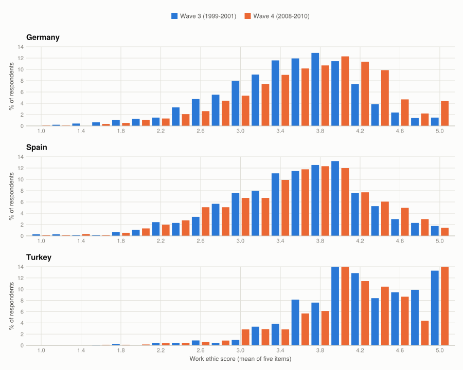
(c) What changed. All three moved up, by very different amounts.
- Germany moved most. The mode went from 3.8 to 4.0 and the mean from 3.48 to 3.73. Both tails shifted: the share scoring 4.4 or above rose from 9.1% to 21.2% while the share at 3.0 or below fell from 26.5% to 17.9%.
- Spain barely moved (3.56 to 3.59). Its mode went the other way, 4.0 down to 3.8, and the distribution widened slightly at both ends — the ≥4.4 share rose from 12.3% to 15.4% with the ≤3.0 share flat at about 24%.
- Turkey is a different distribution altogether: centred near 4.2, strongly left-skewed, and in wave 4 the mode is the 5.0 ceiling itself. The share giving the maximum on all five items doubled, from 13.3% to 26.0%.
function distribution_stats(country, wave)
    f = work_ethic_freq(country, wave)
    w = weights(f.frequency)
    total = sum(f.frequency)
    (mean = round(mean(f.score, w), digits = 2),
     sd = round(std(f.score, w; corrected = false), digits = 2),
     mode = f.score[argmax(f.frequency)],
     pct_high = round(100 * sum(f.frequency[f.score .>= 4.4 - 1e-9]) / total, digits = 1),
     pct_low = round(100 * sum(f.frequency[f.score .<= 3.0 + 1e-9]) / total, digits = 1),
     pct_at_ceiling = round(100 * last(f.frequency) / total, digits = 1))
end

shift = DataFrame(country = String[], wave = String[], mean = Float64[], sd = Float64[],
                  mode = Float64[], pct_high = Float64[], pct_low = Float64[],
                  pct_at_ceiling = Float64[])
for country in P2_COUNTRIES, (i, wave) in enumerate(WAVES[3:4])
    push!(shift, (country, "wave $(i + 2)", distribution_stats(country, wave)...))
end
shift
6×8 DataFrame
| Row | country | wave | mean | sd | mode | pct_high | pct_low | pct_at_ceiling |
|---|---|---|---|---|---|---|---|---|
| String | String | Float64 | Float64 | Float64 | Float64 | Float64 | Float64 | |
| 1 | Germany | wave 3 | 3.48 | 0.68 | 3.8 | 9.1 | 26.5 | 1.5 |
| 2 | Germany | wave 4 | 3.73 | 0.7 | 4.0 | 21.2 | 17.9 | 4.4 |
| 3 | Spain | wave 3 | 3.56 | 0.69 | 4.0 | 12.3 | 23.9 | 1.8 |
| 4 | Spain | wave 4 | 3.59 | 0.71 | 3.8 | 15.4 | 24.1 | 1.4 |
| 5 | Turkey | wave 3 | 4.18 | 0.59 | 4.0 | 41.0 | 3.5 | 13.3 |
| 6 | Turkey | wave 4 | 4.27 | 0.63 | 5.0 | 49.5 | 5.5 | 26.0 |
The Turkish ceiling is a measurement problem, not a finding. When a quarter of respondents give the maximum on every item, the scale has stopped distinguishing between them, and any further strengthening of attitudes cannot show up. Turkey’s mean is censored from above, so 4.27 is a lower bound on where the distribution would sit on an unbounded scale — and the country whose work ethic the hypothesis most relies on is the one where the measure works least well.
Ten years is one wave, and the movements are small against individual variation. Germany’s 0.25 shift is the largest of the three and amounts to roughly a third of the within-country standard deviation of 0.70. The gap between Germany and Turkey in the same wave is 0.54 — twice Germany’s movement across two decades.
Q2. Life satisfaction over four waves
(a) Mean life satisfaction by wave, for countries surveyed in all four.
waves_per_country = combine(groupby(clean, :S003),
                            :S002EVS => (x -> length(unique(x))) => :waves)
const ALL_FOUR = sort(waves_per_country[waves_per_country.waves .== 4, :S003])

life_sat = DataFrame(country = ALL_FOUR)
for (i, w) in enumerate(WAVES)
    life_sat[!, "wave$i"] = [round(mean(clean[(clean.S003 .== c) .& (clean.S002EVS .== w),
                                              :A170]), digits = 2) for c in ALL_FOUR]
end
life_sat.change = round.(life_sat.wave4 .- life_sat.wave1, digits = 2)
sort!(life_sat, :change)
11×6 DataFrame
| Row | country | wave1 | wave2 | wave3 | wave4 | change |
|---|---|---|---|---|---|---|
| String | Float64 | Float64 | Float64 | Float64 | Float64 | |
| 1 | Germany | 7.22 | 7.03 | 7.43 | 6.77 | -0.45 |
| 2 | Sweden | 8.03 | 7.99 | 7.62 | 7.68 | -0.35 |
| 3 | Ireland | 7.82 | 7.88 | 8.21 | 7.82 | 0.0 |
| 4 | Iceland | 8.05 | 8.01 | 8.08 | 8.07 | 0.02 |
| 5 | Northern Ireland | 7.66 | 7.88 | 8.07 | 7.82 | 0.16 |
| 6 | Denmark | 8.21 | 8.17 | 8.31 | 8.41 | 0.2 |
| 7 | Netherlands | 7.75 | 7.77 | 7.83 | 7.99 | 0.24 |
| 8 | Belgium | 7.37 | 7.6 | 7.42 | 7.63 | 0.26 |
| 9 | France | 6.71 | 6.77 | 6.98 | 7.05 | 0.34 |
| 10 | Spain | 6.6 | 7.15 | 6.97 | 7.29 | 0.69 |
| 11 | Italy | 6.65 | 7.3 | 7.18 | 7.4 | 0.75 |
Only 11 of 46 countries appear in all four waves, all of them in Western Europe. The EVS expanded eastward after 1990, so the balanced panel is not a sample of Europe — it is a sample of the countries rich enough to have been surveyed in 1981.
(b) One line per country.
const HIGHLIGHT = ["Germany", "Spain", "Sweden"]

fig = Figure(size = (900, 520))
ax = Axis(fig[1, 1];
          title = "Eleven countries, four decades, a range of 1.6 points",
          ylabel = "Mean life satisfaction (1-10)",
          xlabel = "Survey wave",
          xticks = (1:4, ["1\n1981-84", "2\n1990-93", "3\n1999-2001", "4\n2008-10"]),
          limits = ((0.85, 4.9), (6.2, 8.7)))

for row in eachrow(life_sat)
    row.country in HIGHLIGHT && continue
    lines!(ax, 1:4, [row.wave1, row.wave2, row.wave3, row.wave4];
           color = GRIDLINE, linewidth = 2)
    text!(ax, 4.06, row.wave4; text = row.country, fontsize = 10,
          align = (:left, :center), color = MUTED)
end

for (i, country) in enumerate(HIGHLIGHT)
    row = only(eachrow(life_sat[life_sat.country .== country, :]))
    values = [row.wave1, row.wave2, row.wave3, row.wave4]
    lines!(ax, 1:4, values; color = series_color(i), linewidth = 2.5)
    scatter!(ax, 1:4, values; color = series_color(i))
    # Ink, not the series colour: the coloured line and dot beside the label already
    # carry identity, and slot 3 sits below the 3:1 contrast floor for text.
    text!(ax, 4.06, row.wave4; text = country, fontsize = 11,
          align = (:left, :center), color = INK, font = :bold)
end

fig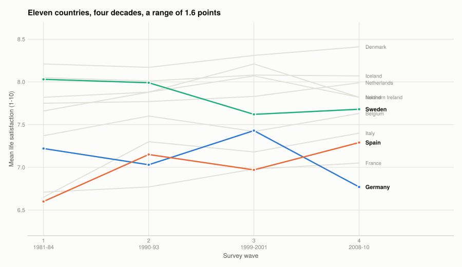
(c) What the averages do and do not show. The dominant feature is how little moves. Denmark and Iceland sit near 8.1–8.4 for thirty years; France near 6.7–7.1. The country ranking is nearly fixed, and the cross-country spread (about 1.6 points) is far larger than any country’s movement over four waves.
Within that, three things are visible:
- Spain and Italy rose most (+0.69 and +0.75 from wave 1 to wave 4), both from low starting points, both over the decades of their post-1980 convergence.
- Germany fell 0.45, and the path is not a trend — 7.22, 7.03, 7.43, 6.77. The wave-4 value is the lowest of the four and the drop from wave 3 is 0.66, the largest single-wave move in the table.
- Sweden fell 0.35, entirely between waves 2 and 3 (7.99 → 7.62).
What a mean of a 1–10 ordinal scale hides, and what would supplement it:
- The distribution. A mean of 7.0 is produced both by everyone answering 7 and by half answering 4 and half answering 10. The share below some threshold — say the proportion answering 5 or less — measures something a mean cannot, and is the quantity relevant to welfare.
- Spread. Standard deviations here run from about 1.7 to 3.1 across countries. Two countries with equal means and that difference in spread are not in the same state.
- Composition. The samples are not the same people, and not even the same kind of people — the population ages between waves, and Q3 shows life satisfaction correlates with age, health and income. Some of the wave-to-wave movement is a changing sample.
- Precision. Nothing above has an interval attached. With 300–1,700 respondents per country per wave, a standard error on a mean is roughly 0.05–0.13, so a 0.1-point move is not distinguishable from noise. This is what Part 8.3 fixes.
(d) Events behind two of these. Germany’s fall between waves 3 and 4 has an obvious candidate: the wave-4 fieldwork (2008–2010) sits on the financial crisis, and German unemployment had risen through the Hartz reforms of 2003–2005 to a post-reunification peak near 11% in 2005. The German figures back this up specifically — unemployment among wave-4 German respondents is 11.2%, and their mean life satisfaction is 4.61, the lowest of any employment group in any of the 46 countries. A large and unusually miserable unemployed group is enough to move a national average.
Spain’s rise from 6.60 to 7.29 spans its entry into the European Communities in 1986, two decades of income convergence, and the construction boom. Wave 4 caught Spain in 2008–2010, when unemployment was climbing past 20% — yet the average was still at its highest. Whatever drove the long rise was strong enough to survive the crisis, which is a caution against reading these averages as a business-cycle indicator.
Q3. Correlations
(a) Employment status and sex are text, so the correlation table needs numeric versions first. Full-time employment is coded 1 for full-time, 0 for unemployed, and missing for the other six statuses — the variable is a contrast between two groups, not an employment indicator, so retired and part-time respondents must be excluded rather than coded 0.
wave4.full_time = [s == "Full time" ? 1.0 : s == "Unemployed" ? 0.0 : missing
                   for s in wave4.X028]
wave4.female = [s == "Female" ? 1.0 : 0.0 for s in wave4.X001]

const CORR_VARS = ["A170" => "Life satisfaction", "work_ethic" => "Work ethic",
                   "X003" => "Age", "Education_1" => "Education",
                   "full_time" => "Full-time employment", "female" => "Female",
                   "A009" => "Self-reported health", "X047D" => "Income",
                   "X011_01" => "Number of children", "percentile" => "Relative income"]

function pairwise_cor(a, b)
    ok = .!ismissing.(wave4[!, a]) .& .!ismissing.(wave4[!, b])
    round(cor(Float64.(wave4[ok, a]), Float64.(wave4[ok, b])), digits = 3)
end

DataFrame(variable = last.(CORR_VARS),
          life_satisfaction = [pairwise_cor("A170", c) for (c, _) in CORR_VARS],
          work_ethic = [pairwise_cor("work_ethic", c) for (c, _) in CORR_VARS],
          observations = [sum(.!ismissing.(wave4[!, c]) .& .!ismissing.(wave4.A170))
                          for (c, _) in CORR_VARS])
10×4 DataFrame
| Row | variable | life_satisfaction | work_ethic | observations |
|---|---|---|---|---|
| String | Float64 | Float64 | Int64 | |
| 1 | Life satisfaction | 1.0 | -0.034 | 49823 |
| 2 | Work ethic | -0.034 | 1.0 | 49823 |
| 3 | Age | -0.082 | 0.133 | 49823 |
| 4 | Education | 0.094 | -0.145 | 49823 |
| 5 | Full-time employment | 0.184 | -0.027 | 24891 |
| 6 | Female | -0.021 | -0.048 | 49823 |
| 7 | Self-reported health | 0.376 | -0.073 | 49823 |
| 8 | Income | 0.235 | -0.152 | 49823 |
| 9 | Number of children | -0.017 | 0.089 | 49823 |
| 10 | Relative income | 0.296 | -0.187 | 49823 |
All ten pairs match the book’s printed values to the last digit it shows.
(b) Reading the coefficients. Signs first, because the coding decides them.
Life satisfaction. The largest correlate is self-reported health at 0.376 — bigger than income, bigger than employment, bigger than anything else measured. Two caveats: both are self-reports collected in the same interview, so a respondent’s general disposition inflates the correlation, and causation runs both ways.
Relative income (0.296) correlates more strongly than raw income (0.235). The percentile is a monotone transformation of income, so a change in correlation is a change in functional form: it says the linear-in-euros specification is wrong, and satisfaction responds more nearly to rank or to log income than to absolute amounts. The pooled percentile also picks up cross-country income differences, so part of the increase is between-country variation, not a better within-country measure.
Full-time employment (0.184) is positive as coded: full-time (1) is more satisfied than unemployed (0). Note its observation count — 24,891 against 49,823 for every other row, because six of the eight statuses are excluded by construction.
Age (−0.082) and children (−0.017) are both small and negative. The age relationship is the well-documented U-shape, and a linear correlation is the wrong summary of it: a coefficient near zero is consistent with a strong non-linear relationship, and this is a case where the number understates what is there.
Work ethic. Its correlation with life satisfaction is −0.034 — effectively zero. This is the single most important number in the table for this project, because it says work ethic is not a proxy for wellbeing at the individual level. Whatever the country-level relationship in Q4 turns out to be, it is not an artefact of happier people having stronger work attitudes.
Work ethic’s own correlates all point one way: education −0.145, relative income −0.187, income −0.152, age +0.133. Stronger work ethic goes with being older, less educated, and poorer. That is a coherent picture — the measure is tracking something like traditionalism — and it is also a warning for Q4, because those characteristics are correlated with the country someone lives in. A cross-country correlation of work ethic with anything else risks picking up national income instead.
Q4. Does the employment gap track work ethic?
(a) and (b) Mean life satisfaction by country and employment status, for the three statuses of interest, and the two differences: D1 = full-time minus unemployed, D2 = full-time minus retired.
const CATS = ["Full time", "Retired", "Unemployed"]

gaps = DataFrame(country = String[], work_ethic = Float64[], full_time = Float64[],
                 retired = Float64[], unemployed = Float64[], D1 = Float64[], D2 = Float64[])
for c in sort(unique(wave4.S003))
    rows = wave4[wave4.S003 .== c, :]
    groups = [Float64.(rows[coalesce.(rows.X028 .== s, false), :A170]) for s in CATS]
    any(g -> length(g) < 2, groups) && continue
    means = mean.(groups)
    push!(gaps, (c, mean(skipmissing(rows.work_ethic)), means...,
                 means[1] - means[3], means[1] - means[2]))
end
sort!(gaps, :work_ethic)
show_all(transform(gaps, names(gaps, Not(:country)) .=> ByRow(x -> round(x, digits = 2));
                   renamecols = false))
46×7 DataFrame
| Row | country | work_ethic | full_time | retired | unemployed | D1 | D2 |
|---|---|---|---|---|---|---|---|
| String | Float64 | Float64 | Float64 | Float64 | Float64 | Float64 | |
| 1 | Iceland | 2.81 | 8.2 | 8.45 | 7.23 | 0.97 | -0.24 |
| 2 | Netherlands | 3.15 | 8.04 | 7.95 | 7.0 | 1.04 | 0.09 |
| 3 | Sweden | 3.25 | 7.88 | 8.17 | 6.52 | 1.36 | -0.3 |
| 4 | Finland | 3.27 | 7.82 | 8.02 | 5.77 | 2.05 | -0.2 |
| 5 | Great Britain | 3.29 | 7.53 | 7.93 | 6.03 | 1.51 | -0.4 |
| 6 | Northern Ireland | 3.31 | 7.68 | 7.77 | 7.54 | 0.14 | -0.09 |
| 7 | Belgium | 3.31 | 7.72 | 7.83 | 6.37 | 1.35 | -0.12 |
| 8 | Croatia | 3.41 | 7.31 | 6.48 | 7.17 | 0.14 | 0.83 |
| 9 | Switzerland | 3.45 | 8.04 | 8.12 | 5.76 | 2.28 | -0.08 |
| 10 | France | 3.47 | 7.2 | 6.97 | 6.24 | 0.96 | 0.23 |
| 11 | Ireland | 3.47 | 7.9 | 7.83 | 7.18 | 0.71 | 0.07 |
| 12 | Poland | 3.5 | 7.46 | 6.57 | 7.06 | 0.4 | 0.89 |
| 13 | Latvia | 3.5 | 6.52 | 5.93 | 5.31 | 1.21 | 0.59 |
| 14 | Denmark | 3.54 | 8.54 | 8.21 | 7.2 | 1.34 | 0.34 |
| 15 | Malta | 3.54 | 7.7 | 7.76 | 5.95 | 1.75 | -0.06 |
| 16 | Bosnia Herzegovina | 3.55 | 7.33 | 7.01 | 6.77 | 0.56 | 0.33 |
| 17 | Estonia | 3.55 | 6.93 | 6.25 | 4.97 | 1.95 | 0.67 |
| 18 | Lithuania | 3.56 | 6.59 | 5.63 | 4.53 | 2.06 | 0.96 |
| 19 | Norway | 3.58 | 8.19 | 8.26 | 8.0 | 0.19 | -0.07 |
| 20 | Spain | 3.59 | 7.34 | 7.21 | 7.19 | 0.15 | 0.13 |
| 21 | Belarus | 3.62 | 6.1 | 5.62 | 5.61 | 0.49 | 0.48 |
| 22 | Russian Federation | 3.62 | 6.86 | 5.7 | 6.4 | 0.46 | 1.16 |
| 23 | Czech Republic | 3.63 | 7.3 | 6.89 | 6.07 | 1.24 | 0.42 |
| 24 | Serbia | 3.67 | 7.17 | 6.67 | 6.73 | 0.44 | 0.5 |
| 25 | Slovenia | 3.68 | 7.83 | 7.13 | 6.76 | 1.07 | 0.7 |
| 26 | Luxembourg | 3.68 | 7.87 | 8.24 | 5.5 | 2.37 | -0.37 |
| 27 | Montenegro | 3.71 | 7.63 | 7.22 | 7.47 | 0.16 | 0.42 |
| 28 | Austria | 3.72 | 7.44 | 7.74 | 6.07 | 1.36 | -0.31 |
| 29 | Germany | 3.73 | 7.26 | 6.85 | 4.61 | 2.65 | 0.41 |
| 30 | Italy | 3.73 | 7.43 | 7.44 | 6.6 | 0.83 | -0.01 |
| 31 | Ukraine | 3.74 | 6.34 | 5.44 | 4.95 | 1.4 | 0.9 |
| 32 | Greece | 3.82 | 7.15 | 6.62 | 5.98 | 1.17 | 0.53 |
| 33 | Slovakia | 3.83 | 7.47 | 6.71 | 6.12 | 1.35 | 0.76 |
| 34 | Macedonia | 3.85 | 7.19 | 6.67 | 6.61 | 0.58 | 0.52 |
| 35 | Hungary | 3.85 | 6.65 | 5.89 | 4.86 | 1.79 | 0.76 |
| 36 | Romania | 3.87 | 7.14 | 6.57 | 7.41 | -0.27 | 0.56 |
| 37 | Northern Cyprus | 3.88 | 6.74 | 6.44 | 5.64 | 1.1 | 0.29 |
| 38 | Armenia | 3.89 | 6.04 | 4.85 | 5.46 | 0.58 | 1.18 |
| 39 | Moldova | 3.9 | 7.12 | 5.98 | 6.07 | 1.05 | 1.14 |
| 40 | Portugal | 3.9 | 6.84 | 5.88 | 5.44 | 1.4 | 0.96 |
| 41 | Albania | 3.92 | 6.63 | 5.81 | 6.07 | 0.57 | 0.83 |
| 42 | Georgia | 3.99 | 6.12 | 4.69 | 5.42 | 0.7 | 1.43 |
| 43 | Cyprus | 4.07 | 7.38 | 7.03 | 6.56 | 0.82 | 0.35 |
| 44 | Kosovo | 4.07 | 6.3 | 6.04 | 6.78 | -0.49 | 0.26 |
| 45 | Bulgaria | 4.12 | 6.18 | 4.97 | 4.69 | 1.48 | 1.2 |
| 46 | Turkey | 4.27 | 6.5 | 6.61 | 5.76 | 0.74 | -0.11 |
All 46 countries have at least two respondents in each of the three groups. Spot checks against the solutions: Great Britain 7.53 / 7.93 / 6.03, Spain 7.34 / 7.21 / 7.19, Turkey 6.50 / 6.61 / 5.76, Germany 7.26 / 6.85 / 4.61 — all exact.
The full-time/unemployed gap is positive in 44 of 46 countries. The two exceptions are Kosovo (−0.49) and Romania (−0.27), where the unemployed report higher satisfaction than full-time workers. The full-time/retired gap is far more mixed: negative in 13 countries, where the retired are the more satisfied group.
Whether social norms explain this cannot be settled by the table. What the table does establish is that the gap is not a fixed quantity: it ranges from −0.49 to +2.65 in Germany, a spread larger than the entire cross-country range of national average life satisfaction. Something country-specific is at work. Candidates other than norms: the generosity of unemployment insurance, the duration of unemployment spells, and how selective unemployment is — where 2% are unemployed they are a different sort of person than where 30% are.
(c) Each difference against country work ethic.
fig = Figure(size = (960, 460))
panels = [(:D1, "Full-time minus unemployed", 1), (:D2, "Full-time minus retired", 2)]

for (col, label, i) in panels
    ax = Axis(fig[1, i];
              title = label,
              xlabel = "Country mean work ethic",
              ylabel = i == 1 ? "Difference in mean life satisfaction" : "",
              limits = ((2.7, 4.4), (-0.8, 2.9)))
    hlines!(ax, [0]; color = BASELINE, linewidth = 1, linestyle = :dash)
    scatter!(ax, gaps.work_ethic, gaps[!, col]; color = series_color(1))
    for country in ["Great Britain", "Spain", "Turkey", "Germany"]
        row = only(eachrow(gaps[gaps.country .== country, :]))
        text!(ax, row.work_ethic, row[col]; text = country, fontsize = 10,
              align = (:center, :bottom), offset = (0, 7), color = INK_SECONDARY)
    end
end

fig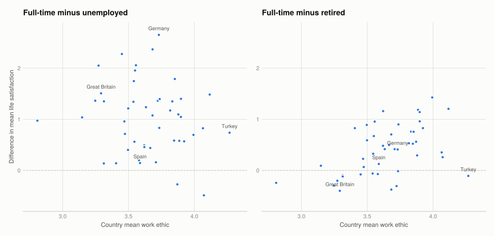
(d) The correlations, and what they do to the hypothesis.
DataFrame(difference = ["D1: full-time minus unemployed", "D2: full-time minus retired"],
          correlation_with_work_ethic = round.([cor(gaps.D1, gaps.work_ethic),
                                                cor(gaps.D2, gaps.work_ethic)], digits = 4),
          countries = nrow(gaps))
2×3 DataFrame
| Row | difference | correlation_with_work_ethic | countries |
|---|---|---|---|
| String | Float64 | Int64 | |
| 1 | D1: full-time minus unemployed | -0.1576 | 46 |
| 2 | D2: full-time minus retired | 0.4843 | 46 |
Both reproduce the book’s walk-through exactly (−0.1575654 and 0.4842609).
D1 is −0.158 — the wrong sign for the hypothesis. The paper’s prediction is that where the work norm is stronger, being unemployed costs more, so D1 should rise with work ethic. In this cross-section it falls slightly. The relationship is weak enough that with 46 countries it is not distinguishable from zero, so the honest statement is: this data provides no support for the hypothesis, rather than evidence against it.
The scatter shows why, and it is not subtle. The high-work-ethic countries in wave 4 are Turkey, Bulgaria, Kosovo, Cyprus, Georgia, Albania and Moldova, and several of them have unemployment above 25%. Where unemployment is a mass condition it is both less stigmatising and less selective, which pushes D1 down exactly where work ethic is highest. The two effects are confounded by construction, and the Q3 finding that work ethic correlates −0.19 with relative income is the same problem in individual-level form: work ethic is partly a proxy for being poor, and poor countries have high unemployment.
D2 is +0.484 — strong, and in the direction norms predict. Where the work ethic is stronger, the retired are much worse off relative to full-time workers; where it is weakest, the retired are more satisfied (Great Britain −0.40, Austria −0.31, Luxembourg −0.37). This is the more interesting result, and it is the comparison where the norm argument should be weakest — the introduction argues that norms of working apply less to the elderly.
Two readings, and this data cannot separate them:
- Norms extend to the retired. In strongly pro-work societies, leaving work is itself costly, so retirement carries some of the same penalty as unemployment.
- Pensions, not norms. High-work-ethic countries here are poorer countries with weaker pension systems. The retired are worse off because they have less money.
Reading (2) is the more parsimonious one given that work ethic correlates −0.15 with income at the individual level, and it does not require the norm mechanism at all. D2 correlating three times more strongly than D1 is a signal that the country-level work-ethic variable is carrying national income, which affects the retired directly.
Part 8.3 — Confidence intervals for a difference in means
Every difference in Part 8.2 was a point estimate with nothing attached. A difference of 0.15 in Spain and 1.51 in Great Britain are not comparable until it is known how precisely each was measured.
For a single mean, the standard error is the sample SD over the root of the sample size. For a difference between two independent groups, the standard errors combine in quadrature:
\[\text{SE}(\bar{x}_1 - \bar{x}_2) = \sqrt{\text{SE}_1^2 + \text{SE}_2^2} = \sqrt{\frac{s_1^2}{n_1} + \frac{s_2^2}{n_2}}\]
Independence is what licenses adding the variances, and it holds here — the full-time and unemployed respondents are different people. It would not hold in the paired design of Project 2, where the same subjects generate both groups.
Q1. Three countries, low, middle and high work ethic
From the Q4 table, sorted by work ethic across 46 countries: Great Britain ranks 5th (3.29, bottom third), Spain 20th (3.59, middle third), Turkey 46th (4.27, top). These are the book’s three.
(a) Means, standard deviations and counts.
const P3_COUNTRIES = ["Turkey", "Spain", "Great Britain"]

group_values(country, status) =
    Float64.(wave4[(wave4.S003 .== country) .&
                   coalesce.(wave4.X028 .== status, false), :A170])

ci_inputs = DataFrame(country = String[], status = String[], n = Int[],
                      mean = Float64[], sd = Float64[], se = Float64[])
for country in P3_COUNTRIES, status in CATS
    x = group_values(country, status)
    push!(ci_inputs, (country, status, length(x), round(mean(x), digits = 2),
                      round(std(x), digits = 2), round(std(x) / sqrt(length(x)), digits = 4)))
end
ci_inputs
9×6 DataFrame
| Row | country | status | n | mean | sd | se |
|---|---|---|---|---|---|---|
| String | String | Int64 | Float64 | Float64 | Float64 | |
| 1 | Turkey | Full time | 330 | 6.5 | 2.55 | 0.1403 |
| 2 | Turkey | Retired | 201 | 6.61 | 2.6 | 0.1831 |
| 3 | Turkey | Unemployed | 299 | 5.76 | 3.13 | 0.1812 |
| 4 | Spain | Full time | 377 | 7.34 | 1.7 | 0.0878 |
| 5 | Spain | Retired | 181 | 7.21 | 1.93 | 0.1436 |
| 6 | Spain | Unemployed | 73 | 7.19 | 2.14 | 0.2503 |
| 7 | Great Britain | Full time | 334 | 7.53 | 1.85 | 0.101 |
| 8 | Great Britain | Retired | 289 | 7.93 | 1.98 | 0.1164 |
| 9 | Great Britain | Unemployed | 78 | 6.03 | 2.19 | 0.2475 |
Every mean, SD and count matches the published table. The standard errors show immediately where the imprecision will come from: Great Britain’s unemployed group has 78 respondents against 334 full-time, so its SE is 0.248 against 0.101. The small group dominates the width of the interval, which is why the unemployed comparisons are less precise than the retired ones despite the differences being larger.
(b) The differences, their standard errors and 95% intervals.
const Z = 1.96

ci_table = DataFrame(country = String[], comparison = String[], difference = Float64[],
                     se = Float64[], half_width = Float64[], lower = Float64[],
                     upper = Float64[], excludes_zero = Bool[])
for country in P3_COUNTRIES
    for (other, label) in [("Unemployed", "Full-time - unemployed"),
                           ("Retired", "Full-time - retired")]
        x, y = group_values(country, "Full time"), group_values(country, other)
        diff = mean(x) - mean(y)
        se = sqrt(var(x) / length(x) + var(y) / length(y))
        push!(ci_table, (country, label, round(diff, digits = 3), round(se, digits = 4),
                         round(Z * se, digits = 3), round(diff - Z * se, digits = 3),
                         round(diff + Z * se, digits = 3), abs(diff) > Z * se))
    end
end
ci_table
6×8 DataFrame
| Row | country | comparison | difference | se | half_width | lower | upper | excludes_zero |
|---|---|---|---|---|---|---|---|---|
| String | String | Float64 | Float64 | Float64 | Float64 | Float64 | Bool | |
| 1 | Turkey | Full-time - unemployed | 0.737 | 0.2292 | 0.449 | 0.288 | 1.187 | true |
| 2 | Turkey | Full-time - retired | -0.107 | 0.2307 | 0.452 | -0.559 | 0.345 | false |
| 3 | Spain | Full-time - unemployed | 0.145 | 0.2653 | 0.52 | -0.375 | 0.665 | false |
| 4 | Spain | Full-time - retired | 0.127 | 0.1683 | 0.33 | -0.203 | 0.457 | false |
| 5 | Great Britain | Full-time - unemployed | 1.507 | 0.2673 | 0.524 | 0.983 | 2.031 | true |
| 6 | Great Britain | Full-time - retired | -0.398 | 0.1542 | 0.302 | -0.7 | -0.096 | true |
These match the book’s R walk-through exactly: Great Britain 1.51 ± 0.524 and −0.398 ± 0.302, Spain 0.145 ± 0.520 and 0.127 ± 0.330, Turkey 0.737 ± 0.449 and −0.107 ± 0.452.
(c) Cross-check with a t-test. Welch’s t-test uses the same standard error but a t distribution with estimated degrees of freedom instead of the normal’s 1.96, so the intervals should be marginally wider.
ttest_table = DataFrame(country = String[], comparison = String[], manual = Float64[],
                        welch = Float64[], t = Float64[], df = Float64[], p = Float64[])
for row in eachrow(ci_table)
    other = endswith(row.comparison, "unemployed") ? "Unemployed" : "Retired"
    x, y = group_values(row.country, "Full time"), group_values(row.country, other)
    test = UnequalVarianceTTest(x, y)
    lower, upper = confint(test)
    push!(ttest_table, (row.country, row.comparison, row.half_width,
                        round((upper - lower) / 2, digits = 3),
                        round(test.t, digits = 3), round(test.df, digits = 1),
                        # `digits` would print the smallest p-value as 0.0; `sigdigits`
                        # keeps it readable however small it gets.
                        round(pvalue(test), sigdigits = 2)))
end
ttest_table
6×7 DataFrame
| Row | country | comparison | manual | welch | t | df | p |
|---|---|---|---|---|---|---|---|
| String | String | Float64 | Float64 | Float64 | Float64 | Float64 | |
| 1 | Turkey | Full-time - unemployed | 0.449 | 0.45 | 3.218 | 575.1 | 0.0014 |
| 2 | Turkey | Full-time - retired | 0.452 | 0.453 | -0.464 | 416.4 | 0.64 |
| 3 | Spain | Full-time - unemployed | 0.52 | 0.527 | 0.547 | 90.5 | 0.59 |
| 4 | Spain | Full-time - retired | 0.33 | 0.331 | 0.754 | 318.3 | 0.45 |
| 5 | Great Britain | Full-time - unemployed | 0.524 | 0.53 | 5.638 | 104.1 | 1.5e-7 |
| 6 | Great Britain | Full-time - retired | 0.302 | 0.303 | -2.581 | 593.8 | 0.01 |
The two agree to within 0.01 in every case, and the largest gap is Turkey’s retired comparison (0.452 against 0.453) where the smaller group has 201 respondents. The book’s walk-through prints Turkey’s t-test interval as [0.2873459, 1.1875704], which this reproduces to seven digits.
The p-values add what the intervals imply: Great Britain’s full-time/unemployed difference has p = 1.5 × 10⁻⁷, Turkey’s p = 0.0014, and Spain’s p = 0.59.
WarningThe book’s Solutions page computes these intervals differently — and gets them wrong
The project text states the correct formula, \(\sqrt{s_1^2/n_1 + s_2^2/n_2}\), and the R walk-through implements it. But the Solutions page (Figures 8.15–8.18, built in Excel) uses \(\sqrt{s_1^2 + s_2^2}\) as an “SD of difference in means” and then divides by \(\sqrt{n_1 + n_2}\):
published = DataFrame(
    country = ["Great Britain", "Spain", "Turkey", "Great Britain", "Spain", "Turkey"],
    comparison = repeat(["Full-time - unemployed", "Full-time - retired"], inner = 3),
    published_half_width = [0.28, 0.25, 0.32, 0.21, 0.21, 0.31])

check = DataFrame(country = String[], comparison = String[], sd_combined = Float64[],
                  n_combined = Int[], solutions_half_width = Float64[],
                  correct_half_width = Float64[])
for row in eachrow(ci_table)
    other = endswith(row.comparison, "unemployed") ? "Unemployed" : "Retired"
    x, y = group_values(row.country, "Full time"), group_values(row.country, other)
    sd_combined = sqrt(var(x) + var(y))
    n_combined = length(x) + length(y)
    push!(check, (row.country, row.comparison, round(sd_combined, digits = 2), n_combined,
                  round(Z * sd_combined / sqrt(n_combined), digits = 3), row.half_width))
end
leftjoin(check, published, on = [:country, :comparison])
6×7 DataFrame
| Row | country | comparison | sd_combined | n_combined | solutions_half_width | correct_half_width | published_half_width |
|---|---|---|---|---|---|---|---|
| String | String | Float64 | Int64 | Float64 | Float64 | Float64? | |
| 1 | Great Britain | Full-time - unemployed | 2.86 | 412 | 0.276 | 0.524 | 0.28 |
| 2 | Spain | Full-time - unemployed | 2.73 | 450 | 0.253 | 0.52 | 0.25 |
| 3 | Turkey | Full-time - unemployed | 4.04 | 629 | 0.316 | 0.449 | 0.32 |
| 4 | Great Britain | Full-time - retired | 2.71 | 623 | 0.213 | 0.302 | 0.21 |
| 5 | Spain | Full-time - retired | 2.58 | 558 | 0.214 | 0.33 | 0.21 |
| 6 | Turkey | Full-time - retired | 3.64 | 531 | 0.309 | 0.452 | 0.31 |
solutions_half_width reproduces the published figures to the two decimals they print, so this is the formula they used. It is not the same quantity: dividing a combined SD by \(\sqrt{n_1 + n_2}\) only coincides with the correct expression when the two groups are equal in size and variance, and here they never are — Great Britain’s unemployed group is a quarter the size of its full-time group.
The published intervals are too narrow by 40% to 106%. Great Britain’s full-time/retired interval is printed as ±0.21 when it is ±0.30; Spain’s full-time/unemployed as ±0.25 when it is ±0.52.
None of the six conclusions change, which is why the error survived: every interval that excludes zero still excludes it, and every one that contains zero still contains it. The substantive answers on the Solutions page are right. Only the widths are wrong, and this page uses the text’s formula and the R walk-through’s numbers.
(d) The differences with their intervals.
fig = Figure(size = (860, 500))
ax = Axis(fig[1, 1];
          title = "Full-time workers are more satisfied than the unemployed; against the retired it depends",
          ylabel = "Difference in mean life satisfaction",
          xlabel = "Ordered by country mean work ethic",
          xticks = (1:3, ["Great Britain\n3.29 (low)", "Spain\n3.59 (middle)",
                          "Turkey\n4.27 (high)"]),
          limits = ((0.5, 3.5), (-1.0, 2.3)))
hlines!(ax, [0]; color = BASELINE, linewidth = 1)

const ORDERED = ["Great Britain", "Spain", "Turkey"]
for (j, label) in enumerate(["Full-time - unemployed", "Full-time - retired"])
    rows = [only(eachrow(ci_table[(ci_table.country .== c) .&
                                  (ci_table.comparison .== label), :])) for c in ORDERED]
    positions = collect((1:3) .+ (j == 1 ? -0.19 : 0.19))
    barplot!(ax, positions, [r.difference for r in rows];
             width = 0.34, color = series_color(j), label = label)
    errorbars!(ax, positions, [r.difference for r in rows], [r.half_width for r in rows];
               color = INK_SECONDARY, whiskerwidth = 12, linewidth = 2)
end

Legend(fig[0, 1], ax; orientation = :horizontal, framevisible = false)
fig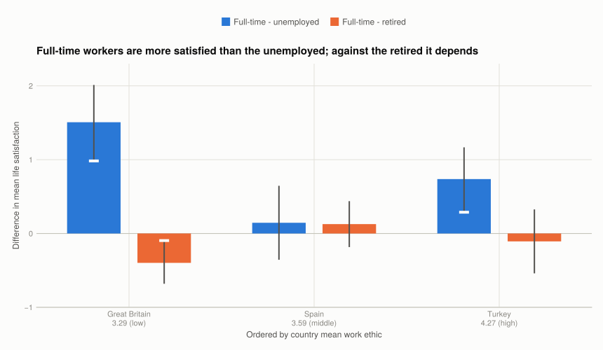
(e) Reading the six intervals. Two clean results, three nulls, and one that matters.
Full-time versus unemployed. All three differences are positive, but only two are distinguishable from zero.
- Great Britain: 1.51 [0.98, 2.03]. The largest gap and the most precisely estimated relative to its size. On a 1–10 scale a point and a half is substantial — comparable to the entire spread between the highest and lowest country averages in the balanced panel.
- Turkey: 0.74 [0.29, 1.19]. Half the British gap, still excludes zero. Turkey’s interval is the narrowest of the three despite the largest standard deviations, because it has 299 unemployed respondents against Great Britain’s 78.
- Spain: 0.15 [−0.38, 0.67]. Indistinguishable from zero. The interval is wide enough to contain both no difference and a gap of two-thirds of a point, so this is uninformative rather than evidence of no difference — a distinction the Solutions’ narrower ±0.25 obscures.
And this is the ordering the hypothesis predicts backwards. Great Britain has the lowest work ethic of the three and the largest gap; Turkey has the highest work ethic and a gap half the size. Spain sits in the middle on work ethic and has no measurable gap at all. Three countries is not a test, but it is the same pattern as the −0.158 correlation across all 46.
Full-time versus retired. Only Great Britain’s differs from zero, and it is negative: −0.40 [−0.70, −0.10], p = 0.010. British retirees are more satisfied than full-time workers. Spain (0.13 [−0.20, 0.46]) and Turkey (−0.11 [−0.56, 0.35]) are both nulls with intervals wide enough to include moderate effects either way.
On precision generally. The half-widths run from 0.30 to 0.52 while the differences run from 0.11 to 1.51 — so the measurement error is the same order of magnitude as most of the effects. Two consequences worth being explicit about:
- The country-level
D1andD2values in Part 8.2 inherit this. Each of those 46 differences carries an interval of roughly ±0.3 to ±0.6, and the correlations of −0.158 and 0.484 were computed as though they were exact. The attenuation from that noise biases both correlations toward zero, which weakens the negativeD1finding and means the trueD2relationship is, if anything, stronger than 0.484. - Precision is driven by the smallest group, not the sample. Wave 4 has 49,823 respondents; these intervals are set by groups of 73 to 78 people. Norway has 7 unemployed respondents and the Netherlands 14 — country-level differences for them are essentially unmeasured, and they entered the Part 8.2 correlations with the same weight as Turkey’s 299.
None of this identifies a causal effect. Unemployment is not assigned at random, and the same characteristics that make someone likely to become unemployed — poor health, low education — independently reduce life satisfaction. The correlation of 0.376 between satisfaction and health is larger than any employment gap here. What would help: a natural experiment such as a plant closure, which makes job loss independent of the individual; or panel data on the same person before and after, which differences out everything fixed about them. The Winkelmann study the project follows uses exactly that panel strategy, which is why it can say more than this cross-section can.
What this project covered
| Concept | Where | In Julia |
|---|---|---|
| Stacking sheets into one frame | Q8.1 Q1 | reduce(vcat, [DataFrame(XLSX.readtable(...))]) |
| Showing every row of a long table | Q8.1 Q6 | show_all(df) — Quarto elides the middle |
Variable labels that survive select |
Q8.1 Q1 | colmetadata!(df, col, "label", v; style = :note) |
String sentinel to missing |
Q8.1 Q3 | comprehension over every column |
| Recoding a verbal scale | Q8.1 Q3 | Dict lookup that throws on an unknown label |
| Splitting one column into two | Q8.1 Q3 | split(v, " : "), then take each part |
| Wave-specific complete cases | Q8.1 Q4 | (wave .!= w) .| ok, checked by per-wave counts |
| Row means across columns | Q8.1 Q5 | mean(Float64[row[c] for c in cols]) |
| Percentiles of a distribution | Q8.1 Q5 | ecdf(x)(x) from StatsBase |
| Pairwise-complete correlation | Q8.2 Q3 | mask both columns, then cor |
| Weighted mean and SD | Q8.2 Q1 | mean(x, weights(w)), std(x, weights(w)) |
| Grey-context emphasis past 8 series | Q8.2 Q2 | grey lines plus 3 coloured, direct-labelled |
| SE of a difference in means | Q8.3 Q1 | sqrt(var(x)/length(x) + var(y)/length(y)) |
| Welch’s t-test | Q8.3 Q1 | UnequalVarianceTTest(x, y), confint, pvalue |
| Error bars on a column chart | Q8.3 Q1 | errorbars!(ax, x, y, half_width) |
The R → Julia page has the full translation table.